SIPAIM 2023
https://doi.org/10.1109/SIPAIM56729.2023.10373416
This is an annotated version of the published manuscript.
Annotations are set as sidenotes, and were not peer reviewed (nor reviewed by all authors) and should not be considered as part of the publication itself. They are merely a way for me to provide some additional context, or mark links to other publications or later results. If you want to cite this article, please refer to the official version linked with the DOI.
Adrien Foucart
In digital pathology, segmentation between tissue and glass slide is a very common pre-processing step in image processing pipelines. It is often presented as relatively trivial, and solved using ad-hoc heuristics that are not always precisely defined nor justified. Most tissue segmentation pipelines start by reducing the color image to a single-channel representation, grayscale being the most common. We show in this study that representations that focus on the colorfulness or entropy offer better separability between tissue and background, and lead to better results in simple thresholding pipelines.
Segmentation of the tissue area from the background glass slide is a common pre-processing step in digital pathology pipelines [1]. The goal of this step is often simply to speed-up the rest of the processing, limiting computationally heavy steps to the tissue area [2]–[4]. It can also serve more specific purposes, such as improving stain estimation for deconvolution or normalisation [5], measuring tissue area for quantification of biomarkers [4] or slide quality control [6], or improving whole-slide registration by excluding non-tissue areas from the optimization process [7]. Despite its prevalence in digital pathology pipelines, this step is often performed using ad-hoc heuristics that do not necessarily generalize well outside of the dataset under study, or provide clear justifications for algorithmic choices. Most tissue segmentation methods use a classical pipeline with a (manual or automatic) threshold on a single-channel image derived from the RGB whole-slide, followed by some post-processing. In this study, we focus on the channel reduction step, and evaluate the impact of this choice on the results of the tissue segmentation. We show that using grayscale or RGB channel averaging, as many studies do, is ill-advised, as it tends to offer far less separability between tissue area and background compared to measures of colorfulness or entropy. Choosing the right channel reduction step leads to robust, state-of-the-art results even with very simple segmentation pipelines. All the code used to produce our results is available at https://gitlab.com/adfoucart/tissue-segmentation.
In a systematic review of artificial intelligence methods for diagnosis in digital pathology, Rodriguez et al. [1] reports many studies that include tissue segmentation as a pre-processing step, noting that “complex techniques do not seem to be very useful", as simple thresholding is generally deemed sufficient. Several studies have focused more specifically on tissue segmentation. In 2015, Bug et al. [3] proposed the FESI algorithm, which converts the image to grayscale, computes the Laplacian, blurs it, then uses various morphological and thresholding techniques to produce the tissue mask. Bandi et al., in 2017 [2] and 2019 [8], proposed a deep learning method based on U-Net to perform the segmentation. Kleczek et al. [5] use the CIELAB color space to perform a color hysteresis thresholding. In 2023, Song et al. [4] proposed EntropyMasker, a method based on the local entropy of the grayscale image.
Comparing the results from those different studies is difficult, given that they all use different datasets, and often focus on different use cases for the tissue segmentation. Instead of trying to optimise a complete pipeline, or to compare pipelines which differ in all their steps, we focus here on the first step of channel reduction, to better understand its impact on the rest of the pipeline. We purposefully chose not to focus on deep learning solutions in this study. Often, one of the objectives of tissue segmentation is to have a very simple and quick method that offer a result that doesn’t need to be pixel-perfect. Making simple, classical pipelines more robust and reliable can allow us to get good results while wasting less computing resources.
There is limited publicly available data that include precise tissue annotations. Bándi et al.’s “representative sample" [9] contains five WSI from their development set and five WSI from their test set, with different tissue regions and stains. The TiGER challenge dataset, available online (https://tiger.grand-challenge.org/), contains 93 H&E stained breast cancer slides from Radboud UMC and Jules Bordet hospital, with the accompanying tissue masks. We use the five WSI from the Bandi et al.’s development set and 62 WSI from the TiGER set as a “development set" to perform a descriptive analysis and to tune the thresholds for the segmentation pipelines, and the remaining slides (5 from Bandi, 31 from TiGER) as a “test set" to validate the results provided by the pipelines using different channels.
All the following experiments are done at a level of magnification corresponding to a resolution of around 15µm/px.
A "channel reduction" step is a transformation from the three channels RGB image to a single channel representation. The goal of this transformation is to achieve a representation such that the tissue and background regions are easily separable. Four different "channel reduction" steps are considered in this study, based on our survey of the state of the art. In all cases and to make comparisons easier, we use the convention that background region correspond to low values and tissue regions to high values in the single channel image.
Grayscale: probably the most commonly used channel reduction (e.g., see [6], [10]–[12]). For this study, we used the definition from scikit-image (\(Y = 0.2125 R + 0.7154 G + 0.0721 B\)). Some studies use the simple average of the RGB channels [12], but we found few differences in results compared to grayscale. We use the inverse grayscale in order to have the tissue brighter than the background.
Saturation: the saturation channel from the HSV color space is a common, simple alternative to the grayscale channel (e.g. [13], [14]). The light gray background region is expected to be desaturated, while the stained tissue region will be saturated.
Color Distance: used in VALIS [15] registration software, this channel reduction step first converts the image to the CAM16UCS color space. It estimates the color of the background based on the brightest pixels in the image using the lightness channel, then computes the euclidean distance in the color space.
Local Entropy: used in EntropyMasker [4], it is similar in concept to others who use the Laplacian [3], [16] or Canny edges [17], as it postulates that background regions will be less textured (and therefore have lower entropy and less edges) than the tissue regions. The local entropy of the grayscale image is computed using as neighbourhood a disk of radius 10px : like the thresholds, this was set based on the results on the development set. --AF .
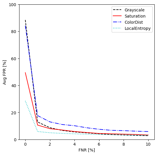
On each image of the development set we computed, for each channel reduction, the separability of the "tissue" and "background" distributions, defined as \(s = \frac{(\mu_{tissue} - \mu_{bg})^2}{\sigma_{tissue}^2+\sigma_{bg}^2}\) (similarly to the separability criterion of Otsu [18]), after applying a median filter with a disk of radius 5px. We also look at the False Positive Rate (FPR, i.e. percentage of background pixels which would be incorrectly identified as tissue) for different levels (steps of 1% between 0-10%) of False Negative Rates (FNR, i.e. percentage of tissue pixels which are missed), based on threshold segmentation. This is done by computing the threshold that leads to each targeted FNR, then computing the corresponding FPR.
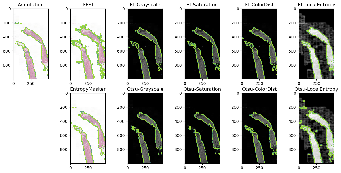
FESI and EntropyMasker are used as state-of-the-art reference algorithms. For each of the four potential channels, we use the same simple pipeline: channel reduction, median filter with a disk of radius 5px, thresholding, and post-processing by filling the holes followed by a morphological opening with a disk of radius 5px. The holes in the annotated tissue mask (generally corresponding to tissue tears or vessels) are also filled, as whether or not it’s useful to include them is highly dependent on the application. Two options are considered for thresholding: using the Otsu algorithm (commonly used in the surveyed literature [16], [19]–[21]), or using a fixed threshold. The latter is set for each channel separately as the threshold that maximises the Intersection over Union (IoU) between the pixels above the threshold and the pixels in the annotated tissue mask over the development set. For Grayscale, Saturation and ColorDist, which tend to have a trimodal distribution (with the background slide and the two stains having separate peaks), multi-Otsu with three classes is used, and the lowest threshold is selected. Results on the test set are reported using the IoU between the predicted and annotated tissue masks as an all-purpose overlap metric.
| Grayscale | Saturation | ColorDist | LocalEntropy | |
|---|---|---|---|---|
| Median Sep. | 3.46 | 3.61 | 3.68 | 11.63 |
| Interquartile | [1.63-6.30] | [1.81-6.22] | [1.65-7.06] | [7.15-15.05] |
Table 1 shows the separability of the different channels on the development set images. The LocalEntropy channel demonstrates a much higher separability than the other three. A Friedman test on the results show statistically significant difference between the distributions (\(pval < 10^{-15}\)), and the Nemenyi post-hoc test shows LocalEntropy to be significantly different from the other three (\(pval < 10^{-7}\)). Figure 1 shows the average FPR for different fixed FNR values on the development set. While all channels have similar FPR (except for ColorDist which remains a bit higher) once we accept at least 5% FNR, the LocalEntropy shows lower FPR values at low FNR. At 0% FNR, we can see that we have close to 90% FPR for the Grayscale and ColorDist channels, indicating that there is at least one tissue pixel with a value lower than most background pixels in those channels. No channel offer perfectly separable distributions, with most of the overlap coming either from artefacts in the background (e.g. coverslip or dirty slide) or almost transparent regions in the foreground (e.g. adipose tissue).
| Algorithm | Median IoU | IQ Range |
|---|---|---|
| EntropyMasker | 0.87 | [0.83-0.93] |
| FESI | 0.60 | [0.48-0.80] |
| Grayscale (t=0.026) | 0.83 | [0.64-0.92] |
| Saturation (t=0.029) | 0.93 | [0.88-0.96] |
| ColorDist (t=0.030) | 0.85 | [0.69-0.94] |
| LocalEntropy (t=3.85) | 0.90 | [0.86-0.96] |
| Grayscale (Otsu) | 0.79 | [0.47-0.91] |
| Saturation (Otsu) | 0.83 | [0.58-0.90] |
| ColorDist (Otsu) | 0.88 | [0.52-0.92] |
| LocalEntropy (Otsu) | 0.81 | [0.75-0.91] |
Table 2 reports the IoU computed on the test set for the two reference methods (EntropyMasker and FESI) and the much simpler pipelines involving one of the four channel reductions, either with the learned, fixed thresholds or using Otsu thresholding. A Friedman test showed a significant difference (\(pval < 10^{-12}\)) between the distributions. The Nemenyi post-hoc test shows that the best results (Saturation with fixed threshold) are not significantly different (\(pval > 0.05\)) from EntropyMasker, LocalEntropy and ColorDist : using the confidence interval on rankings method that we introduced at ESANN 2025, this is equivalent to saying that those four (bolded) methods have "1" in their ranking CI and are therefore reasonably likely to be "the best". --AF , the latter two with a fixed threshold. FESI appears to perform poorly on these data. (Multi-)Otsu thresholding is generally less reliable than the fixed thresholds. Results on a representative image of the test set (i.e. with an IoU value close to the median for each pipeline) are shown in Figure 2.
Our results demonstrate that transforming the RGB image to grayscale, as is very commonly done for tissue segmentation, is a suboptimal choice that should generally be avoided. Better channel reduction choices are available, focusing either on the colorization of the tissue compared to the background (e.g. with Saturation or ColorDist), or on the texture (e.g. with LocalEntropy). Pipelines with many handcrafted steps such as the one proposed in EntropyMasker may be unecessarily complex, as a very simple pipeline obtain very similar results as long as the right channel reduction step is applied.
There are two main limitations to this study. The first one is that the main source of available annotated tissue masks is the TiGER dataset, which focuses only on H&E stained breast tissue. While some diversity is provided by the Bándi dataset (both in terms of tissue type and staining agents), it includes fewer images. Having more detailed annotations for a diversity of sources would allow for a more detailed analysis. The second main limitation is that, as we focused on the channel reduction aspect, we may miss some interactions between the channel choice and the rest of the pipeline. The separability experiment, however, shows that there is a fundamental advantage to using texture-based information such as the local entropy.
Still, several future experiments should be done to get a better understanding of all the algorithmic choices in tissue segmentation, and answer questions such as: which channels can be combined together to improve the segmentation quality? How much impact can we measure from the choices in pre- or post-processing steps?
Tissue segmentation is often overlooked as a rather trivial step in digital pathology image processing. Our research shows, however, that there are many algorithmic choices that can alter its results. Since this step is so often a part of digital pathology pipelines, gaining a better understanding of the effects of those choices can help build more reliable pipelines for a variety of applications.
This research was supported by the Walloon Region (Belgium) in the framework of the PIT program Prother-wal under grant agreement No. 7289. CD is a senior research associate with the National (Belgian) Fund for Scientific Research (F.R.S.-FNRS) and is an active member of the TRAIL Institute (Trusted AI Labs, https://trail.ac/, Fédération Wallonie-Bruxelles, Belgium). CMMI is supported by the European Regional Development Fund and the Walloon Region (Walloniabiomed, #411132-957270, project “CMMI- ULB”).