SNOW data in digital pathology - Supplementary materials
Adrien Foucart*, Olivier Debeir, Christine Decaestecker
Adrien Foucart*, Olivier Debeir, Christine Decaestecker
| Label | Operation | Kernel Size | Output Tile Size |
Output #Channels |
|---|---|---|---|---|
| Input | N | 3 | ||
| C1 | Conv2D(Input) | 3x3 | N | 64 |
| R1_1 | Conv2D(C1) | 3x3 | N | 64 |
| R1_2 | Conv2D(R1_1) | 3x3 | N | 64 |
| R1_3 | Conv2D(R1_2) | 3x3 | N | 64 |
| R1_A | Add(C1, R1_3) | N | 64 | |
| R1 | MaxPool2D(R1_A) | 2x2 | N/2 | 64 |
| R2_1 | Conv2D(R1) | 3x3 | N/2 | 64 |
| R2_2 | Conv2D(R2_1) | 3x3 | N/2 | 64 |
| R2_3 | Conv2D(R2_2) | 3x3 | N/2 | 64 |
| R2 | Add(R1,R2_3) | N/2 | 64 | |
| R3_1 | Conv2D(R2) | 3x3 | N/2 | 64 |
| R3_2 | Conv2D(R3_1) | 3x3 | N/2 | 64 |
| R3_3 | Conv2D(R3_2) | 3x3 | N/2 | 64 |
| R3_A | Add(R2,R3_3) | N/2 | 64 | |
| R3 | MaxPool2D(R3_A) | 2x2 | N/4 | 64 |
| U1 | Conv2D_Transpose(R3) | 2x2 | N/2 | 64 |
| R4_1 | Conv2D(U1) | 3x3 | N/2 | 64 |
| R4_2 | Conv2D(R4_1) | 3x3 | N/2 | 64 |
| R4_3 | Conv2D(R4_2) | 3x3 | N/2 | 64 |
| R4 | Add(U1,R4_3) | N/2 | 64 | |
| U2 | Conv2D_Transpose(R3) | 2x2 | N | 64 |
| R5_1 | Conv2D(U2) | 3x3 | N | 64 |
| R5_2 | Conv2D(R5_1) | 3x3 | N | 64 |
| R5_3 | Conv2D(R5_2) | 3x3 | N | 64 |
| R5 | Add(U2,R5_3) | N | 64 | |
| C2 | Conv2D(R5) | 1x1 | N | 2 |
| Output | Softmax(C2) | N | 2 |
| Label | Operation | Kernel Size | Output Tile Size |
Output #Channels |
|---|---|---|---|---|
| Identical to ShortRes Baseline until R3 | ||||
| C2 | Conv2D(R3) | 3x3 | N/4 | 16 |
| R4_1 | Conv2D(C2) | 3x3 | N/4 | 16 |
| R4_2 | Conv2D(R4_1) | 3x3 | N/4 | 16 |
| R4_3 | Conv2D(R4_2) | 3x3 | N/4 | 16 |
| R4_A | Add(C2,R4_3) | N/4 | 16 | |
| R4 | MaxPool2D(R4_A) | 2x2 | N/8 | 16 |
| U1 | Conv2D_Transpose(R4) | 2x2 | N/4 | 16 |
| U2 | Conv2D_Transpose(U1) | 2x2 | N/2 | 16 |
| Output | Conv2D_Transpose(U2) | 2x2 | N | 3 |
| Label | Operation | Kernel Size | Output Tile Size |
Output #Channels |
|---|---|---|---|---|
| Input | N | 3 | ||
| R1_1 | Conv2D(Input) | 3x3 | N | 64 |
| R1_2 | Conv2D(R1_1) | 3x3 | N | 64 |
| R1_S | Conv2D(Input) | 1x1 | N | 64 |
| R1_A | Add(R1_S, R1_2) | N | 64 | |
| R1 | MaxPool2D(R1_A) | 2x2 | N/2 | 64 |
| R2_1 | Conv2D(R1) | 3x3 | N/2 | 128 |
| R2_2 | Conv2D(R2_1) | 3x3 | N/2 | 128 |
| R2_S | Conv2D(R1) | 1x1 | N/2 | 128 |
| R2_A | Add(R2_S,R2_2) | N/2 | 128 | |
| R2 | MaxPool2D(R2_A) | 2x2 | N/4 | 128 |
| R3_1 | Conv2D(R2) | 3x3 | N/4 | 256 |
| R3_2 | Conv2D(R3_1) | 3x3 | N/4 | 256 |
| R3_S | Conv2D(R2) | 1x1 | N/4 | 256 |
| R3_A | Add(R3_S,R3_2) | N/4 | 256 | |
| R3 | MaxPool2D(R3_A) | 2x2 | N/8 | 256 |
| R4_1 | Conv2D(R3) | 3x3 | N/8 | 512 |
| R4_2 | Conv2D(R4_1) | 3x3 | N/8 | 512 |
| R4_S | Conv2D(R3) | 1x1 | N/8 | 512 |
| R4 | Add(R4_S,R4_2) | N/8 | 512 | |
| U1_1 | Conv2D_Transpose(R4) | 2x2 | N/4 | 256 |
| U1_2 | Conv2D(U1_1) | 3x3 | N/4 | 256 |
| U1_S | Conv2D_Transpose(R4) | 1x1 | N/4 | 256 |
| U1 | Add(U1_S,U1_2) | N/4 | 256 | |
| U2_C | Concat(U1,R2) | N/4 | 384 | |
| U2_1 | Conv2D_Transpose(U2_C) | 2x2 | N/2 | 128 |
| U2_2 | Conv2D(U2_1) | 3x3 | N/2 | 128 |
| U2_S | Conv2D_Transpose(U2_C) | 1x1 | N/2 | 128 |
| U2 | Add(U2_S,U2_2) | N/2 | 128 | |
| U3_C | Concat(U2,R1) | N/2 | 192 | |
| U3_1 | Conv2D_Transpose(U3_C) | 2x2 | N | 64 |
| U3_2 | Conv2D(U3_1) | 3x3 | N | 64 |
| U3_S | Conv2D_Transpose(U3_C) | 1x1 | N | 64 |
| S1 | Add(U3_S,U3_2) | N | 64 | |
| S2 | Resize(U2) | N | 128 | |
| S3 | Resize(U1) | N | 256 | |
| F1 | Conv2D(S1) | 1x1 | N | 2 |
| F2 | Conv2D(S2) | 1x1 | N | 2 |
| F3 | Conv2D(S3) | 1x1 | N | 2 |
| F_A | Add(F1,F2,F3) | N | 2 | |
| F | Conv2D(F_A) | 1x1 | N | 2 |
| Output | Softmax(F) | N | 2 |
| Label | Operation | Kernel Size | Output Tile Size |
Output #Channels |
|---|---|---|---|---|
| Identifcal to PAN Baseline until U1 | ||||
| S | Resize(U1) | N | 256 | |
| Output | Conv2D(S) | 1x1 | N | 3 |
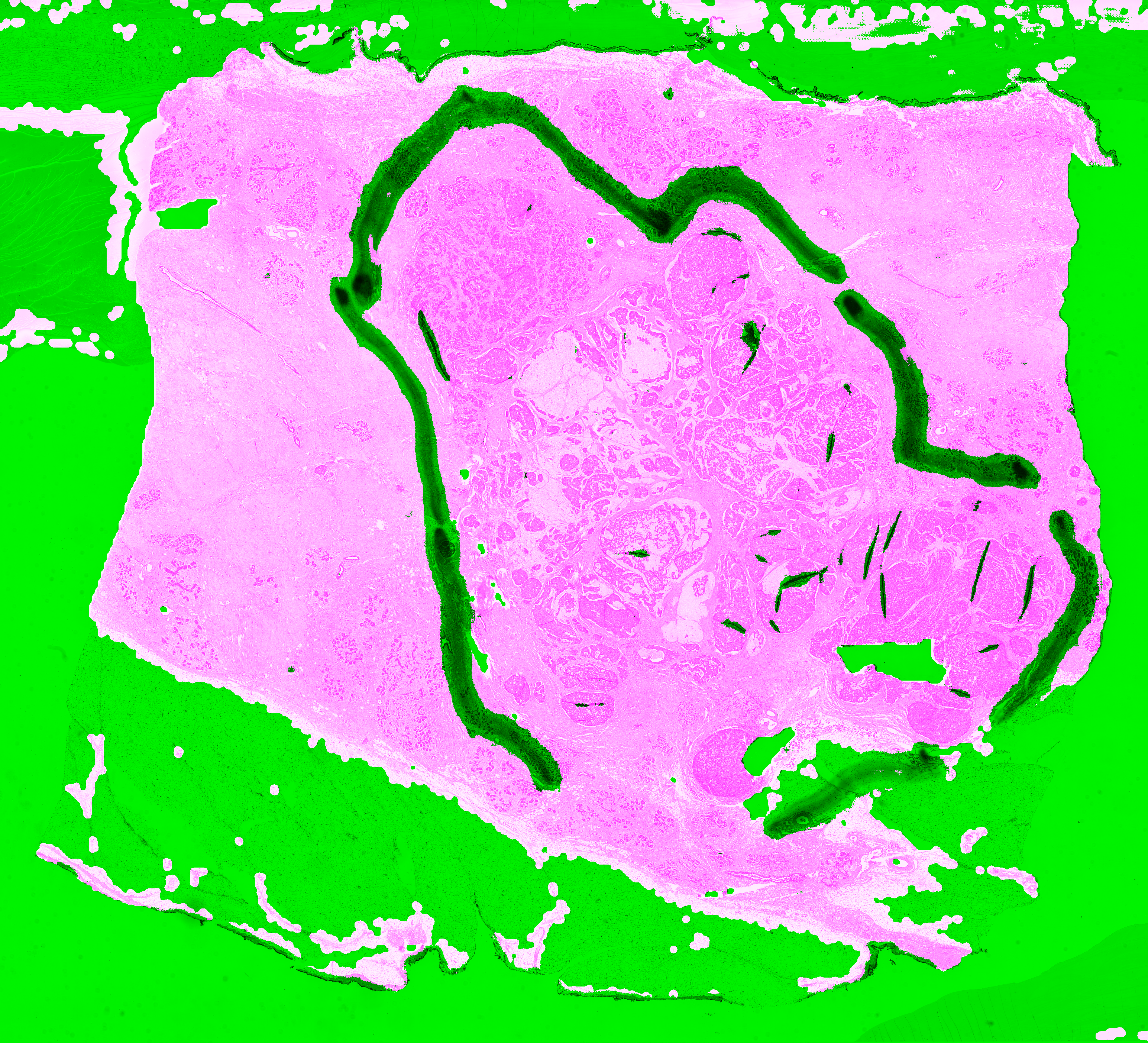
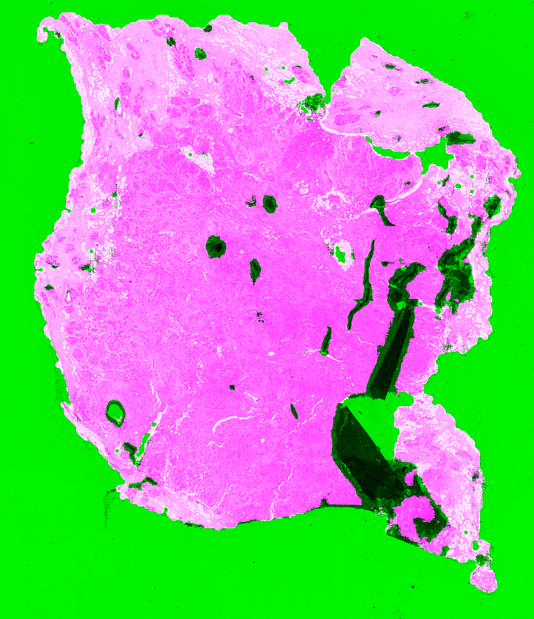
Segmentation results of the PAN-GA50 network (PAN using the Generated Annotations strategy with a 50% chance of using the output of the generator as annotation on negative patches during training). Normal tissue is colored in pink and artefacts are colored in green.
| Block C |
|---|
 |
| TCGA A1-A0SQ |
 |
| TCGA AC-A2FB |
 |
| TCGA AO-A0JE |
 |
| TCGA D8-A141 |
 |
Flowchart illustrating the process for analyzing a dataset through the SNOW framework.

To get the download link to the artefact dataset, please contact Adrien Foucart: afoucart@ulb.ac.be
The corrupted noisy datasets were created by removing a certain percentage of the annotated objects from the supervision. As objects can vary in size, we verify on the corrupted GlaS dataset that we don't introduce a biais in some of the datasets by only removing small or big objects. The following graph shows the percentage of pixels removed from the annotations as a function of the percentage of objects removed.
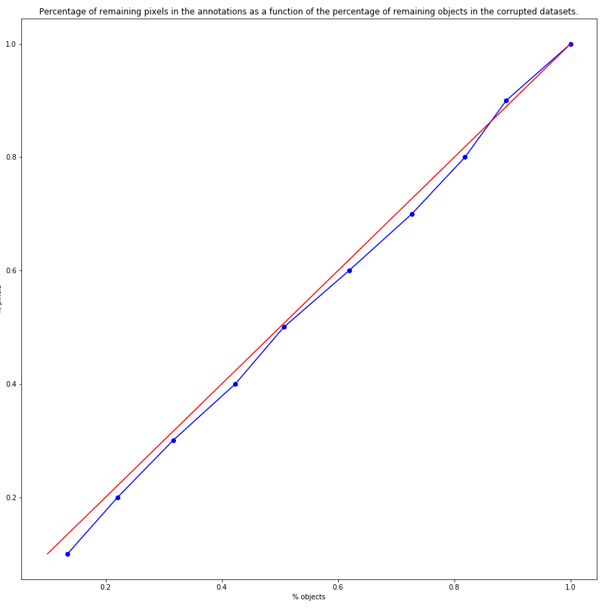
| Corrupted Dataset | % objects remaining | % pixels remaining |
|---|---|---|
| 10% noise | 89.47% | 88.93% |
| 20% noise | 78.93% | 81.84% |
| 30% noise | 69.18% | 72.70% |
| 40% noise | 58.39% | 61.90% |
| 50% noise | 47.33% | 50.66% |
| 60% noise | 38.10% | 42.34% |
| 70% noise | 28.48% | 31.59% |
| 80% noise | 18.47% | 22.08% |
| 90% noise | 11.05% | 13.45% |