[Devlog] Supervoxel CT liver segmentation

I have some micro-CT images of mice, where I need to segment the liver. I haven’t done a lot of 3D image processing before, and after spending a few years in the “deep learning” side of the force, I thought it would be nice to look at some good classic image processing methods and to see how I could use them. The images are not too hard, because a contrast product was injected in the mice before the acquisition, so that the liver is a bit brighter than other soft tissues in the images.

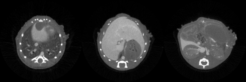
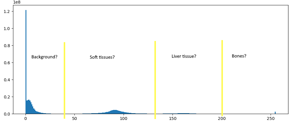
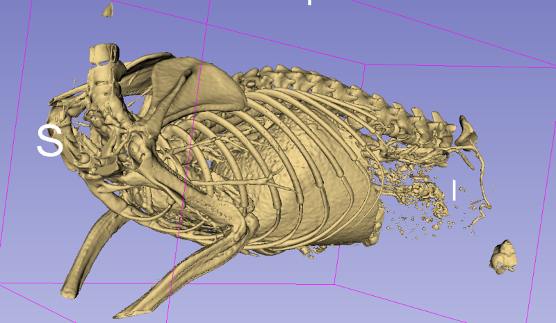
It’s not quite as easy as doing a binary thresholding, however. If we look at the histogram of the whole volume with values scaled between 0 and 255, we seem to have four main distributions, which mostly correspond to background, soft tissue, contrasted soft tissue, and bones. The distributions, however, are very much overlapping. So if we try to just take “natural” thresholds manually, like here 130 and 200, we end up taking a lot of bones and missing some actual liver tissue. Not ideal.

A method that I’ve always liked in 2D are “superpixels,” where you start by making a regular grid that is deformed so that it sticks to the borders in the image, creating large irregular but mostly homogeneous “pixels.” What’s interesting when you do that is that your “new” image is a lot “smaller” (so easier to process) while keeping the most useful information (where the borders are) intact. In 3D, we don’t have pixels, we have voxels, but the process can still apply. And reducing the size of the image in a clever way like “supervoxels” seems like it could be really useful in 3D images, as the processing time can quickly become very large. This is not a particularly original idea: I quickly checked, and found a paper from 2016 that basically had most of the pipeline that I had in mind (Wu et al. 2016) for the same application (in humans, though). I’m going to simplify things a little bit however, as the presence of the contrast product makes it a little bit easier to find the region of interest.

The pipeline I tested is as follows:

• Compute supervoxels with SLIC
• Create graph connecting neighbours, and compute basic stats per supervoxel (mean intensity, volume)
• Filter out supervoxels outside of expected range of mean intensity values for the liver
• Iteratively merge neighbours of similar intensities.
• Select largest merged supervoxel as “liver” segment.

Let’s have a look at what we can get.

SLIC supervoxels

SLIC is a commonly used algorithm for finding superpixels (or, in 3D, supervoxels) (Achanta et al. 2012). I use here the implementation from the SimpleITK library, which is relatively straightforward:

slic = sitk.SLIC(volume, 
                 superGridSize=(grid_size, grid_size, grid_size),
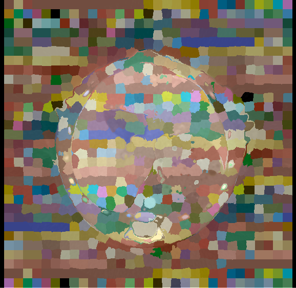
                 spatialProximityWeight=proximity_weight)

It has two main parameters to play with: the size of the “super grid,” which will determine how many superpixels there are, and the “spatial proximity weight,” which will determine whether the resulting grid will be “more regular” or if you allow more deformations. Here, I have set the grid size to 20x20x20, and the proximity weight to 20.0. As we can see in the figure, in homogeneous regions (like in the background), the supervoxels tend to be very regular, while in regions with more borders they deform to adapt to the local information.

Computing the graph

After the previous step, we have a 3D volume with, for each voxel, a label so that every voxel that has the same lable belongs to the same supervoxel. We want to have a “graph” of how those supervoxels are connected together, so we need to find their neighbours. The simplest way of doing that is to iterate through the supervoxels, dilate them, and find all the other supervoxels that intersect with the dilated volume:

# note: slic here has been converted to a numpy array
idxs = np.unique(slic)
for idx in idxs:
    mask = volume == idx
    neighbours = list(np.unique(slic[dilation(mask, el)]))
    neighbours.remove(idx) # remove current supervoxel from list of neighbours

And we can at the same time compute the average intensity value of the region in the volume, and save all that meta-information in a dedicated structure. The problem with this simple approach is that it takes a lot of time: for each supervoxel, we need to make a binary comparison and a morphological operation on the entire volume. And in 3D, things scale up very fast. Without the morphological operation, running this code would already take about 5-6h on my computer. To speed things up, we go through the volume by more reasonable chunks of around 20x20x20 voxels, updating the supervoxel information and the neighbours lists as we go along:

for z in range(0, volume.size.z, window_size):
    for y in range(0, volume.size.y, window_size):
        for x in range(0, volume.size.x, window_size):
            chunk_slic = slic[z:z + window_size, y:y + window_size, x:x + window_size]
            chunk_volume = volume_array[z:z + window_size, y:y + window_size, x:x + window_size]
            idxs = np.unique(chunk_slic)
            for idx in idxs:
                if idx not in supervoxels:
                    supervoxels[idx] = Supervoxel(idx=idx, total=0, volume=0)

                mask = chunk_slic == idx
                neighbours = list(np.unique(chunk_slic[dilation(mask, el)]))
                supervoxels[idx].add(total=chunk_volume[mask].sum(),
                                     volume=np.count_nonzero(mask),
                                     neighbours=neighbours)
                supervoxels[idx].add_chunk(IntVector(x=x, y=y, z=z),
                                           IntVector(x=x+window_size, y=y+window_size, z=z+window_size))

This allows us to go from 5 hours to around 30 seconds without the morphological operation, and around 3 minutes with it for a full volume. This could be further accelerated with some multithreading, but I don’t really need the speed at the moment, so that exercise will be left for another time.

Now that we have our graph, we can also filter any supervoxel that has a mean value outside of the expected range. Ideally, this range should be computed automatically, but for the moment I just use the 130-200 range that I previously defined.

Iterative merging

For the last part of the method, I use a much simpler heuristic than the “graph cut” from (Wu et al. 2016). First, I build a list of all connections between neighbours, sorted based on the absolute difference in mean values. The first “connection” will therefore be between the two neighbouring supervoxels that are the most similar in terms of mean intensity. These two supervoxels are then “merged”: the smallest of the two is “consumed” by the largest (and its neighbours list is also merged with the other’s). Then we iterate through the sorted list of connections.

Two additional parameters control this merging process: a MAX_VOLUME, so that we don’t merge two supervoxels if it would result in an object that’s too large, and a MAX_DISS so that, when we reach a connection that has a dissimilarity above a given threshold (I used 10 in my experiments), we stop.

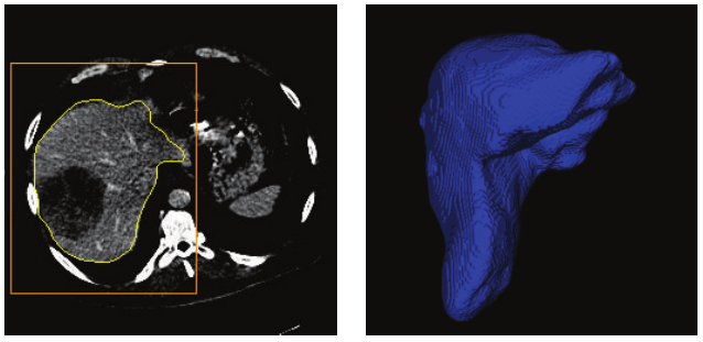
We then consider that the largest remaining supervoxel is our target object.

Conclusion

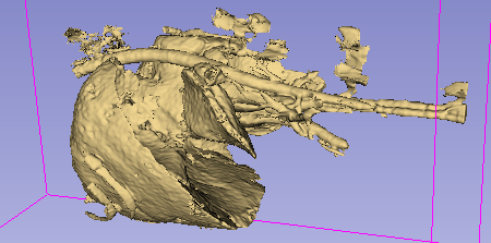
The result is still a bit noisy, but I’m very happy with it given the overall simplicity of the approach. The main difficulty will probably come from the large… artery, I think? Basically: the contrast agent used to highlight the tissue is also present in the vascular system, and it’s therefore difficult to avoid taking part of that system along. It should however be possible to use some post-processing to detect regions where we are in a “tubular” shape, and filter them out.

For such “specialized” applications, creating the kind of datasets needed for deep learning methods would be extremely challenging, so it’s really interesting I think to keep some “old school” methods alive. There is still a fair amount of work required to make the pipeline more robust - and to validate it - but I think it works well as a proof-of-concept.

References