Computerized Medical Imaging and Graphics 2023
https://doi.org/10.1016/j.compmedimag.2022.102155
This is an annotated version of the published manuscript.
Annotations are set as sidenotes, and were not peer reviewed (nor reviewed by all authors) and should not be considered as part of the publication itself. They are merely a way for me to provide some additional context, or mark links to other publications or later results. If you want to cite this article, please refer to the official version linked with the DOI.
Adrien Foucart
Digital pathology image analysis challenges have been organised regularly since 2010, often with events hosted at major conferences and results published in high-impact journals. These challenges mobilise a lot of energy from organisers, participants, and expert annotators (especially for image segmentation challenges). This study reviews image segmentation challenges in digital pathology and the top-ranked methods, with a particular focus on how ground truth is generated and how the methods’ predictions are evaluated. We found important shortcomings in the handling of inter-expert disagreement and the relevance of the evaluation process chosen. We also noted key problems with the quality control of various challenge elements that can lead to uncertainties in the published results. Our findings show the importance of greatly increasing transparency in the reporting of challenge results, and the need to make publicly available the evaluation codes, test set annotations and participants’ predictions. The aim is to properly ensure the reproducibility and interpretation of the results and to increase the potential for exploitation of the substantial work done in these challenges.
In 2010, the Pattern Recognition in Histopathological Image Analysis (PR in HIMA) challenge was held at the 20th International Conference on Pattern Recognition (ICPR) conference [1]. Competing algorithms were evaluated on the tasks of lymphocytes detection and segmentation in breast cancer tissue, and centroblasts detection in follicular lymphoma. Five teams participated in this challenge, which is the first competition focusing on digital pathology tasks [2], [3]. Digital pathology challenges have become a standard component of large biomedical imaging conferences such as the Medical Image Computing and Computer Assisted Intervention Society (MICCAI) conference or the IEEE International Symposium on Biomedical Imaging (ISBI). Their results are now often published in impactful journals, and are often seen as a critical validation step for image analysis methods [2].
The segmentation (and classification) of histological structures is an important step in the automated analysis of histological slides [4]. The required creation of ground truth annotations for segmentation datasets and the evaluation of segmentation algorithms, however, are challenging by themselves. Manual annotation of histological objects is a time-consuming and error-prone task [3], [5], and segmentation metrics are subject to potential biases [6] and to limitations due to inter-expert disagreement [7].
The aim of this review is to analyse how segmentation challenges in digital pathology have managed the above mentioned issues, and to examine the results and insights gained from the winning methods in light of the limitations of both the annotations and evaluation processes : The analysis of challenges regarding the use of metrics was extended to detection and classification challenges in my PhD dissertation. --AF . We examine how the ground truth annotations were created, which evaluation metrics were selected, how the ranking was performed in cases where multiple metrics were used, as well as the level of transparency provided by the challenge organisers, involving in particular the the public release of information such as the evaluation code, the detailed prediction maps from the participants, or the individual annotations from multiple experts. We will also look more closely at a few selected examples that provided us with particularly interesting insights.
A review of digital pathology challenges was published in 2020 [3]. It focused on the value of these challenges to the pathology community with regards to the type of images and of organs studies. The authors highlight a disconnect between the most studied histological objects in clinical practice and in image analysis challenges, and the danger of using datasets from a small number of centres and acquisition devices.
A 2018 critical analysis of biomedical challenges and their rankings [2] demonstrated the lack of robustness of challenge rankings with regard to small variations in the metrics used, in the results aggregation methodology, in the selection of experts for the annotations and in the selection of the teams that are ranked. We previously studied the importance of taking inter-expert disagreement into account in the evaluation of challenges using the Gleason 2019 challenge [7].
A 2021 review of AI in digital pathology [8] examines how deep learning methods can be included in immuno-oncology workflows, looking at challenges and at publications using deep learning for digital pathology. The authors identify the key issues of generalisation capabilities, explainability, and data quality and quantity as challenges to overcome for deep learning to be included in fully validated digital pathology systems.
Other reviews have been made on deep learning methods for biomedical imaging in general [9], [10], and in histopathology in particular [11], [12]. They typically focus on the adaptations of the typical deep learning and computer vision pipelines to the specificities of biomedical image modalities. Deep learning methods have been found to generally outperform other image processing techniques in all digital pathology tasks for which standard network architectures have been widely adapted from other fields. From these surveys, however, it is very difficult to draw solid conclusions as to whether some architectures perform better than others, or which pre- or post-processing steps consistently lead to better results. Data augmentation, stain normalisation, pre-training, custom loss functions and ensemble methods have been identified as important steps, but the importance of their relative contribution seems to often depend on the specific implementation details.
The study of evaluation metrics and their biases has mostly been covered for classification tasks [13]–[16], but some work has also been done for detection [17] and segmentation [6] metrics. They find that commonly used metrics in challenges and other publications are often subject to large biases, large sensitivity to class imbalances, and asymmetrical responses to false positive and false negative errors. For segmentation metrics, for instance, the Dice Similarity Coefficient (DSC) doesn’t penalise under- and over-segmentation equivalently, and is very unstable for small objects : IoU has the same problem: it's more an "overlap metric" than a specific DSC issue. --AF , while the unbounded nature of the Hausdorff Distance (HD) makes it difficult to use it when aggregating multiple cases, particularly in the presence of missing values (such as unmatched objects). Combining different metrics in a single score is also found to be complicated, and often requires arbitrary choices in the weighting or normalising of the different components of the score. We demonstrated in a previous work the possible impact of using entangled metrics that evaluate multiple sub-tasks at the same time compared to using independent metrics, based on the MoNuSAC 2020 challenge results [18].
Challenges were initially identified through the grand-challenge.org website, maintained by Radboud University Medical Center. They were added to this review if they met the following inclusion criteria:
The dataset was composed of histological images (Whole Slide Images, Tissue Microarrays or regions of interest extracted from either).
The task of the challenge included a component of segmentation. Tasks that measured segmentation performance alongside other performances were included, but tasks that focused solely on detection, classification, or clinical diagnosis or prognosis were excluded.
Additional challenges not included in the grand-challenge.org database were found using the list of biomedical challenges compiled in [2], and following through mentions of past challenges in other reviews and publications using previously held challenge datasets. When limited information was found on the challenge website and no result publication was available, peer-reviewed and preprint papers from challenge participants were used to fill in the missing data : It's quite impressive how much information is already missing from competitions that were not held that long ago, and how challenges don't keep their website updated with post-challenge publications. --AF .
For each of the identified challenges, the following information were compiled:
Name and year of organisation.
Host organisation or event and organising team.
Challenge website (or archived version of the website, or in some cases pages from organisations linked to the challenge that provided information about it).
Post-challenge publication of the results.
Number of teams that submitted their results.
Process for creating the ground truth annotations (number of experts and possible consensus method).
Evaluation metrics and ranking process.
Availability of the evaluation source code.
Level of details provided on the teams’ results.
Availability of the inter-expert agreement, if multiple experts were involved.
Source of the dataset’s images.
Information on the methods of the top-3 ranking teams (and publication of the method by their respective authors, if available).
In some cases, particularly for the more recent challenges whose results are not published yet, some of that information is currently restricted to the challenge participants. The information used in this review is based on what is currently publicly available to the research community in general. The inclusion of new challenges into this review was stopped at the end of January 2022.
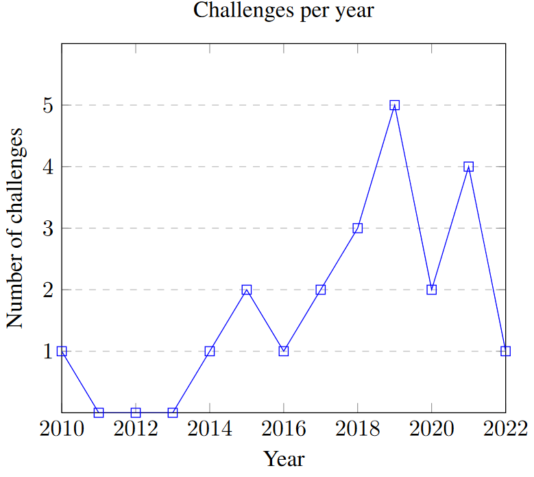
Twenty-one challenges, organised between 2010 and 2022, were included in this review. Of those, eleven have led to a peer-reviewed publication as of January 2022. Seven of the remaining challenges were held in 2019 or after and may therefore lead to publications in the future. The distribution of concerned challenges per year is shown in Fig. 1. Table 1 contains general information about every challenge included in this review. Eleven challenges were hosted at MICCAI or as MICCAI-endorsed events, three at ISBI, four at other conferences (ICPR, ICIAR, KOSOMBE, ISICDM), and three were organised independently. About half of the challenges used data sourced from the The Cancer Genome Atlas2 (TCGA) and The Cancer Imaging Archive3 (TCIA) archives (with annotations provided by experts from the organising team), the others using homemade datasets from organising and partner hospitals. The 2022 Conic challenge uses images from previously published challenges and datasets (DigestPath, CRAG, GlaS, CoNSeP and PanNuke).
| Year | Title | Host | (Segmentation) task(s) | Ref. | Link |
|---|---|---|---|---|---|
| 2010 | PR in HIMA | ICPR | Lymphocytes in regions with lymphocytic infiltration in breast and ovarian cancer samples. | [1] | Web Archive |
| 2014 | Brain Tumour Digital Pathology Challenge | MICCAI CBTC | Necrosis regions in glioblastoma (GBM) tissue. | Web Archive | |
| 2015 | GlaS | MICCAI | Prostate glands in normal and cancer tissue | [19] | Challenge website |
| 2015 | Segmentation of Nuclei in Digital Pathology Images | MICCAI CBTC | Nuclei in selected regions of TCGA Gliomas. | TCIA Wiki | |
| 2016 | Segmentation of Nuclei in Images | MICCAI CPM | Nuclei in selected regions from TCGA cases with different cancer types. | Web Archive | |
| 2017 | Segmentation of Nuclei in Images | MICCAI CPM | Nuclei in selected regions from TCGA cases with different cancer types. | [20] | Web Archive |
| 2018 | Segmentation of Nuclei in Images | MICCAI CPM | Nuclei in selected regions from a set of glioblastoma and lower grade glioma WSI. | [21] | Web Archive |
| 2018 | MoNuSeg | MICCAI | Multi-organ nuclei. | [22] | Challenge website |
| 2018 | BACH | ICIAR | Segmentation of benign, in situ and invasive cancer regions in breast tissue WSI. | [23] | Challenge website |
| 2019 | Gleason | MICCAI | Gland segmentation and grading in prostate cancer. | Challenge website | |
| 2019 | ACDC@LungHP | ISBI | Segmentation of lung carcinoma in WSI. | [24] | Challenge website |
| 2019 | PAIP | MICCAI | Segmentation of tumour region in liver WSI. | [25] | Challenge website |
| 2019 | DigestPath | MICCAI | Colonoscopy tissue segmentation and WSI classification. | [26] | Challenge website |
| 2019 | BCSS | Breast cancer semantic segmentation. | [25] | Challenge website | |
| 2020 | MoNuSAC | ISBI | Multi-organ nuclei detection, segmentation and classification. | [27] | Challenge website |
| 2020 | PAIP | KOSOMBE | Tumour region in colorectal resection WSI and WSI classification. | Challenge website | |
| 2021 | SegPC | ISBI | Multiple myeloma plasma cells segmentation. | [28] | Challenge website |
| 2021 | PAIP | MICCAI | Perineural invasion in resected tumour tissue of the colon, prostate and pancreas. | Challenge website | |
| 2021 | NuCLS | Nuclei detection, segmentation and classification from breast cancer WSI. | [29] | Challenge website | |
| 2021 | WSSS4LUAD | ISICDM | Tumour / stroma / normal tissue segmentation in lung adenocarcinoma. | Challenge website | |
| 2022 | Conic | Nuclei segmentation and classification in colon tissue. | Challenge website |
Organising teams are often involved in multiple challenges, sometimes reusing part of the same dataset and/or annotations in updated versions of the competition. The Tissue Image Analysis Center (formerly TIA Lab) organised the GlaS challenge in 2015 and Conic in 2022, and its founding director, Dr Nasir Rajpoot, was one of the organisers of the “PR in HIMA" challenge in 2010. The laboratory of one of the co-organisers of that challenge, Dr Anant Madabhushi, from Case Western University in Ohio, was also involved in the MoNuSeg and MoNuSAC challenges. Radboud University Medical Center in the Netherlands was involved in the ACDC@LungHP, LYON 2019 (lymphocyte detection) and PANDA 2020 (prostate cancer grading) challenges, as well as the LYSTO (lymphocyte assessment) hackathon (with TIA). They are also the maintainers of the grand-challenge.org website. The Brain Tumour Digital Pathology Challenge in 2014 and the Segmentation of Nuclei in Images from 2015 to 2018 were organised by the Stony Brook’s Department of Biomedical Informatics. All editions of the PAIP challenge involved Seoul National University Hospital, Korea University and Ulsan National Institute of Science and Technology in South Korea. BCSS and NuCLS are both organised by the same teams from Northwestern University in Chicago, Emory University School of Medicine in Atlanta, and several hospitals and faculties in Cairo, Egypt.
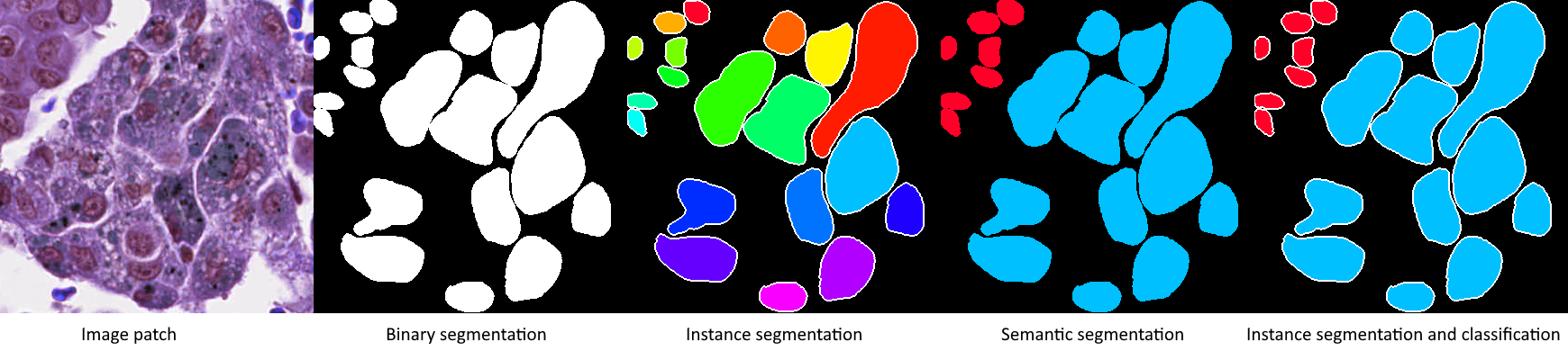
Image analysis tasks can usually be coarsely divided into detection, segmentation and classification. Detection aims to find individual instances of an object of interest. Segmentation is about determining the shape and size of the object or region at the pixel level. Classification focuses on determining the class of an object, region or full image. In digital pathology, grading could also be seen as a type of classification where the classes are ordered. Actual tasks : i.e. tasks that have some real use cases. --AF are often combinations of these broad categories. Instance segmentation combines segmentation with detection, semantic segmentation combines segmentation with classification, and the three can be combined together as instance segmentation and classification (see Fig. 2). The distribution of the challenges according to these categories is reported in Table 2.
An evolution can be seen in the reviewed challenges from simple binary or instance segmentation in earlier challenges, towards semantic segmentation (starting with BACH in 2018) and instance segmentation and classification (starting with MoNuSAC in 2020). The main target objects are nuclei and tumour regions, with various organs represented. Repeat editions of the same challenge tend to keep the same object of interest, but vary the organ (as in the nuclei segmentation of MICCAI CPM or the tumour region segmentation of PAIP) and the scope of the challenge (as in MoNuSAC adding the nuclei classification to the instance segmentation of MoNuSeg). The same evolution is apparent in challenges targeting similar objects and organs from different organisers. For instance, the GlaS challenge in 2015 evaluated algorithms on instance segmentation of colonic glands, while the Gleason challenge in 2019 concerns the grading of prostate cancers, which is based on the glands patterns. Before MoNuSeg, multiple challenges targeted nuclei instance segmentation, and the classification step has been included in the two nuclei segmentation challenges organised after MoNuSAC (NuCLS and Conic). This classification is useful to measure the link between the tumour’s microenvironment (TME) and development [27].
| Task type | # | Challenges |
|---|---|---|
| Binary segmentation | 7 | PR in HIMA 2010, Brain Tumour DPC 2014, ACDC@LungHP 2019, PAIP 2019, DigestPath 2019, PAIP 2020 |
| Instance segmentation | 7 | GlaS 2015, Segmentation of Nuclei in Images 2015-2018, MoNuSeg 2020, PAIP 2021, SegPC 2021 |
| Semantic segmentation | 4 | BACH 2018, Gleason 2019, BCSS 2019, WSS4LUAD |
| Instance segmentation and classification | 3 | MoNuSAC 2020, NuCLS 2021, Conic 2022 |
Digital pathology tasks are known for their high interexpert disagreement [11], including in tasks found in these challenges such as nuclei detection and classification [30], [31] or Gleason grading [32]–[34]. In segmentation tasks, the exact border drawn by an expert may depend on the conditions of the annotation process (software and hardware used), the experience of the expert, or the time assigned to the task, leading to significant interobserver variations [7], [24]. All challenges evaluated their results based on a single ground truth annotation map. It is therefore important to analyse and understand how this ground truth was constructed, and if the differences in participating team’s results are within the range of acceptable interexpert disagreement levels.
There is a big diversity in the strategies used by the challenges. The simple solution of using a single expert as ground truth was used by the PR in HIMA 2010, GlaS and ACDC@LungHP challenges, with the latter using a second expert to assess interobserver variability. They reported an average Dice Similarity Coefficient of 0.8398 between the two experts, very close to the results of the top teams (with the top 3 between 0.7968 and 0.8372).
Several challenges use students (in pathology or in engineering) as their main source of supervision, under the supervision of an expert pathologist reviewing their work. This was the case for the Segmentation of Nuclei in Images challenges of 2017 and 2018 (no information was found for the earlier editions of the challenge), as well as for the MoNuSeg and MoNuSAC challenges.
The Seg-PC challenge in 2021 relied on a single expert for identifying nuclei of interests, then on an automated segmentation method which provided a noisy supervision [28], at least for the training set. It is unclear whether the same process was applied for the test set used for the final evaluation, as that information is not present in the publicly available documents of the challenge.
When using multiple experts, the processes vary and are sometimes left unclear. BACH and PAIP 2019 used one expert to make detailed annotations, and one to check or revise them. DigestPath 2019 and the 2020 and 2021 editions of PAIP all mention “pathologists" involved in the annotation process, but don’t give details on how they interacted and came to a consensus. Gleason 2019 used six different experts who annotated the images independently. A consensus ground truth was automatically generated from their annotation maps using the STAPLE algorithm [35]. BCSS, NuCLS and WSSS4LUAD used a larger cohort of experts and non-expert with varying degrees of experience, with more experienced experts reviewing the annotation of least experienced annotators until a consensus annotation was produced.
Finally, Conic 2022 uses an automated method to produce the initial segmentation, with pathologists reviewing and refining the results.
The three most common metrics for evaluating binary segmentation in segmentation challenges are the Dice Similarity Coefficient (DSC), the Intersection over Union (IoU) and the Hausdorff Distance (HD). Almost all the challenges included in this review use at least one of them. While these simple metrics have clear definitions, they need to be adapted to the assessment of the challenges, which leaves room for variation. Even for simple binary segmentation tasks, the evaluation of a test set requires a choice of how to aggregate measurements made on multiple images, which can be of varying sizes. Additional adaptations, and thus choices, are required in the case of multiple instance segmentation. Indeed, the detection errors should be penalised and the matching between the segmented and ground truth objects should be determined in order to calculate segmentation scores. Furthermore, for the semantic segmentation tasks, an additional choice needs to be made on how to aggregate the per-class results. Instance segmentation and classification tasks combine all those choices: when to aggregate the per-class metrics, how to match prediction and ground truth instances, how to aggregate image-level metrics?
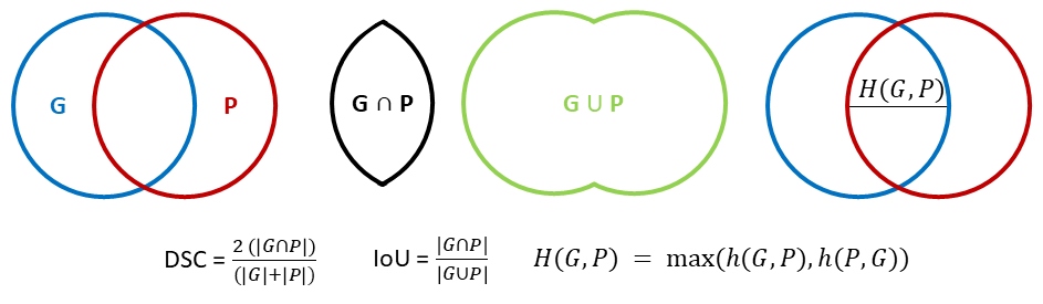
In this section, we formally define the three basic metrics (also illustrated in Fig. 3), and briefly mention the few challenges that used other metrics. We then look at the different strategies used to incorporate instance matching into the evaluation, and the different ways to approach the aggregation process. Finally, we also look at the different ways in which the challenge organisers communicated the results and the evaluation methods actually used. A synthetic view of the different choices made by each challenge regarding the evaluation methods is presented in Table 3.
The DSC [36] is usually defined in binary segmentation problems as:
\[DSC(G,P) = \frac{2 |G \cap P|}{|G| + |P|}\]
Where \(G\) is the ground truth mask, \(P\) the predicted mask, and \(| \cdot |\) denotes the area covered by a mask. This is simply the per-pixel formulation of the F1-score.
The IoU [37] is similarly defined as:
\[IoU(G, P)= \frac{|G \cap P|}{|G \cup P|}\]
It is clear that the two metrics are heavily correlated, and very similar in nature. Both of these metrics are quick to compute, and give an easily interpretable result bounded between 0 (no overlap) and 1 (perfect overlap). They also share two main weaknesses: on small objects, they are extremely sensitive to even single-pixel differences (which is particularly problematic on problems where the object’s exact borders are ill-defined), and they are completely insensitive to shape differences [6].
The HD is defined as:
\[H(G,P) = max(h(G,P), h(P,G))\]
With \(h(A,B) = max_{a \in C_A} min_{b \in C_B} ||a-b||\) and where \(C_A\) is the set of all points in the contour of object A [38]. In plain words, this is the maximum distance between any point on the contour of an object and the closest point in the contour of the other. It is therefore a metric that is very sensitive to the relative shape of the objects, and to the presence of outlier points, as even objects with a significant overlap may end up with large HD if some parts of their contours diverge [39]. This metric is a lot heavier to compute than the DSC and IoU, and is without upper limit, with 0 corresponding to a perfect overlap of the objects.
The DSC, IoU and HD are illustrared in Fig. 3.
The PR in HIMA 2010 challenge also used the Sensitivity (\(SN(G,P) = \frac{|G \cap P|}{|G|}\)), Specificity (\(SP(G,P) = \frac{N - |G \cap P|}{N - |G|}\), where \(N\) is the total number of pixels in the image), Positive Predictive Value (\(PPV(G,P) = \frac{|G \cap P|}{|P|}\)), and the Mean Absolute Distance (MAD) between the two contours (\(MAD(C_G,C_P) = \frac{1}{M} \sum_{p \in C_P} min_{s \in C_S}||p - s||\), where \(M\) is the number of point in the predicted contour \(C_P\)).
In BACH 2018, the classes are treated as an ordered set from 0 (normal tissue) to 3 (invasive carcinoma), and a custom score weighs the errors according to how far the prediction is from the ground truth:
\[s = 1 - \frac{\sum_{i=1}^N |P_i - G_i|}{\sum_{i=1}^N max(G_i, |G_i-3|) \times [1-(1-P_{i,bin})(1-G_{i,bin})] + a}\]
Where \(P_i\) and \(G_i\) are the predicted and ground truth classes of the \(i\)th pixel in an image, \(pred_{i,bin}\) is the “binarized" value of the class, defined as 0 if \(pred_i = 0\) and 1 otherwise, and \(a\) is a “very small number" to avoid division by zero.
Gleason 2019 used a combination of Cohen’s Kappa and F1 scores, and will be discussed more thoroughly in a further section.
PAIP 2019 used a modified “thresholded" IoU, where the IoU is set to 0 if it is lower than 0.65 “to penalise inaccurate results" [25].
In multiple instance segmentation, the basic metrics are typically computed at the object level rather than at the image level. A matching mechanism is therefore necessary to pair ground truth objects with their corresponding predictions. The evaluation method must also determine how to incorporate the “detection" errors (unmatched ground truth or predicted objects) in the overall score.
GlaS 2015 uses the maximum overlap to determine matching pairs (largest area of intersection). The “Detection F1-score" is computed and ranked separately from the “object-level" DSC and HD. This challenge will also be discussed in more detail in a further section.
The Segmentation of Nuclei in Images challenges aggregate the “intersection area" and the “sum of object area" of all pairs of intersecting objects, then use those aggregated values to compute an overall DSC-like score (“Ensemble Dice").
MoNuSeg 2018 uses the maximum IoU as a matching criterion, then also aggregates the “intersection" and “union" over all objects in an image, with “detection" false positives and false negatives being added to the union count (“Aggregated Jaccard Index"). SegPC 2021 also uses the maximum IoU, but chooses to ignore false positives in the metric’s computation.
PAIP 2021 identifies matches based on a combination of bounding box overlap (“two bounding boxes overlap more than 50%") and a maximum HD, and uses the object detection F1-score as a final metric.
MoNuSAC 2020 defines a match as a pair of ground truth and predicted objects with an IoU superior to 0.5. The detection and segmentation performances are merged together into the “Panoptic Quality" metric [40], defined as:
\[PQ(G,P) = F(G,P) \times mIoU(G,P)\]
Where \(F\) is the detection F1 score based on the matching pairs of objects and mIoU is the average IoU of the matching objects’ masks : For details on why that's a bad metric for this task, see my Pattern Recognition paper, my Scientific Reports paper, and my PhD dissertation... --AF .
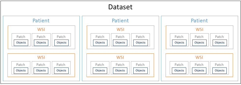
Digital pathology datasets generally have a hierarchical structure illustrated in Fig. 4, composed of patients, whole-slide images (WSI), image patches and, finally the annotated objects if applicable. The metrics are generally computed either at the object level or at the image patches level, and are then aggregated in some way over the whole dataset.
Most challenges first compute or aggregate their chosen metric(s) at the image level, then compute the arithmetic mean over all the images of the test set. In the case of PAIP 2019, the metrics are directly computed on the WSIs.
DigestPath 2019 does not mention the aggregation process. Their test set contains 250 WSIs from 150 patients, so it is unclear whether the results were first averaged per-patient, or if they were directly aggregated over all the slides.
GlaS 2015 aggregates the object-level metrics on the entire test set, with each object’s contribution to the final score weighted by its area.
Challenges that incorporate a classification aspect (i.e. semantic segmentation) generally compute their metric(s) initially per-class. BCSS 2019 reports an “overall" result for all classes, without clearly explaining how it was computed. WSSS4LUAD similarly reports per-class results and both a “mean" and “frequency weighted" average, without clearly defining how exactly those are computed. MoNuSAC 2020 aggregates the per-class scores for each image, then aggregates the per-image scores on the test set, while the Conic Challenge 2022 takes the opposite approach by first aggregating the per-image scores for each class, then computing the final score as the average of the per-class scores.
The main method used to report challenge results is generally through the leaderboard published on the challenge website, which often only reports the final aggregated score and the corresponding ranking. Several challenges go beyond that in the post-challenge publication and provide extra transparency on their results in different ways.
ACDC@LungHP 2019 and PAIP 2019 provided boxplots showing the distribution of results on the test set for the top-10 and top-9 teams respectively. MoNuSeg 2018 provided the averaged results with their 95% Confidence Interval for each of the 32 participants, as well as more detailed per-organ results. Gleason 2019 published the confusion matrices for the per-pixel grade predictions of the top-8 teams. MoNuSAC 2020 released a visualisation of the prediction masks of four of the top-5 teams (excluding the winner) on all test set images.
The evaluation codes for the Glas 20154, MoNuSeg 20185, MoNuSAC 20206, SegPC 20217 and Conic 20228 challenges were publicly released.
It is interesting to note that, whenever more detailed information is available, it tends to offer a much more nuanced view on the results that a simple ranking would suggest. For instance, the box-plots show near-identical distributions for the top teams in the challenges that published them, and the confusion matrices of the Gleason 2019 challenge show that the results may be heavily influenced by how the class imbalance was managed and how the per-class results were aggregated (which is not very clear in that particular case).
| Challenge | Basic metric(s) | Adaptation(s), aggregation, remarks |
|---|---|---|
| PR in HIMA 2010 | DSC, IoU, HD, Sensitivity, Specificity, PPV, MAD | Every metric computed separately. Average of per-image scores. |
| Brain Tumour Digital Pathology Challenge 2014 | DSC | “Positive" class varies depending on whether necrosis tissue is present or not in the ground truth image. Average of per-image scores. |
| GlaS 2015 | F1 score (detection), DSC, HD | Maximum overlap object matching. Average of per-object scores. |
| Segmentation of Nuclei in Images 2015-2018 | DSC | Combines simple binary DSC with “Ensemble Dice" (detailed in the main text). Average of per-image scores. |
| MoNuSeg 2018 | IoU | Detection included in the “Aggregated Jaccard Index" (detailed in the main text). Average of per-image scores. |
| BACH 2018 | Custom score | Unclear if average of per-image scores or if score is computed directly on all pixels of the test set. |
| Gleason 2019 | F1 score, Cohen’s Kappa | Average of per-image scores. |
| ACDC@LungHP 2019 | DSC | Average of per-image scores. |
| PAIP 2019 | IoU | “Thresholded" IoU. Average of per-WSI scores. |
| DigestPath 2019 | DSC | Unclear. |
| BCSS 2019 | DSC | Computed per-class, unclear how final scores are aggregated. |
| MoNuSAC 2020 | PQ | Average of per-image scores. Per-image scores are the average of per-class scores. |
| PAIP 2020 | IoU | Unclear. |
| SegPC 2021 | IoU | Average of per-instance (cell) scores. False positives are ignored. |
| PAIP 2021 | F1 score (detection) | HD used to determine matches. |
| NuCLS 2021 | IoU, DSC (+ diverse detection & classification metrics) | Median of per-image scores. |
| WSSS4LUAD 2021 | IoU | Computed per-class, aggregation method unclear. |
| Conic 2022 | PQ | Average of per-class scores. Per-class scores are the average of per-image scores. |
Thirty-three methods were collected and analysed from fourteen different challenges, based on the availability of the methods information. For some methods, only a broad description in the overall challenge results publication was available. Others were described in short papers on ArXiV or available from the challenge website. Finally, some individual methods led to more detailed peer-reviewed publications (or were re-using a method described in a previously published paper). All methods used in this analysis are listed in Table 4. When specific mention of a method is made in the text, it will be referenced as “Challenge Year #Rank" (for instance, “GlaS 2015 #2" refers to the method ranked second in the GlaS 2015 challenge).
| Challenge | Rank | Source of the method information |
|---|---|---|
| PR in HIMA 2010 | 1 | Conference proceedings [41] |
| 2 | Conference proceedings [42] | |
| 3 | Conference proceedings [43] | |
| GlaS 2015 | 1 | Main publication [19], winning method [44] |
| 2 | Main publication | |
| 3 | Main publication, previous publication [45] | |
| Seg. of Nuclei in Images 2017 | 1 | Main publication [20] |
| Seg. of Nuclei in Images 2018 | 2 | Main publication [21] |
| MoNuSeg 2018 | 1 | Supplementary materials of main publication [22] (Zhou et al) |
| 2 | Supplementary materials (Li J) | |
| 3 | Supplementary materials (Hu Z) | |
| BACH 2018 | 1 | Conference proceedings [46] |
| 2 | Conference proceedings [47] | |
| Gleason 2019 : there's also now a publication from the winning team in Frontiers in Oncology [Qiu et al.] --AF | 1 | Github |
| ACDC@LungHP 2019 | 1 | Main publication [24] |
| 2 | idem | |
| 3 | idem + post-challenge publication [48] | |
| PAIP 2019 | 1 | Main publication [25] |
| 2 | idem | |
| 3 | idem | |
| DigestPath 2019 | 1 | Post-challenge publication [26] |
| MoNuSAC 2020 | 1 | Supplementary materials of main publication [27] (L1), previously published method [49] |
| 2 | Supplementary materials (L2) | |
| 4 | Supplementary materials (PL2) | |
| PAIP 2020 | 1 | Workshop extended abstracts |
| 2 | idem | |
| 3 | idem | |
| SegPC 2021 | 1 | ArXiV [28] |
| 2 | Post-challenge publication [50] | |
| 3 | ArXiV [51] | |
| PAIP 2021 | 1 | Workshop extended abstracts |
| 2 | idem | |
| 3 | idem |
The methods used in the “PR in HIMA 2010" challenge stand out as a snapshot of “classical" image analysis approaches, before Deep Learning algorithms became ubiquitous. They are still interesting in retrospect by illustrating how they adapt the classic image processing pipeline to the characteristics of digital pathology images. The top 3 methods all use the sparsity of the pathology colour space to make the process easier: PR in HIMA 2010 #1 use the mean-shift algorithm to reduce the number of colours, so that a simple HSV thresholding can be applied to segment candidate nuclei. #2 performs a PCA in RGB space to reduce the colour information to a single channel, then applies a Gaussian Mixture Model to similarly segment the candidate regions. #3 performs a RGB thresholding with more weight on the red channel, identified as containing most of the staining information. The three methods then use morphological operations and/or prior knowledge on the expected shape of the object to filter candidates and reduce segmentation noise. Shape and colour features are then extracted for each candidate object, which are used to classify the candidate regions into lymphocytes or non-lymphocytes. #1 uses Support Vector Machines, #2 Transferable Belief Model, and #3 uses template matching. Shape information is also used to detect potential overlaps that need to be split, either based on the known average area of the lymphocytes (#1), the eccentricity (#2), or simply with morphological openings (#3).
All the top available methods from the subsequent challenges reviewed here use Deep Learning algorithms. Some of the challenges that those Deep Learning algorithms face when confronted with digital pathology images, remain the same as in PR in HIMA. The importance of the staining agents and their colour information, and the difficulty of managing touching or overlapping objects remain relevant. Deep Learning algorithms also bring their own requirements and challenges with them. In particular, the small size of digital pathology datasets and the difficulty in getting high quality and high quantity annotations are important topics of discussion through all challenges. In the rest of this section, we will examine the different aspects of the Deep Learning pipelines in digital pathology through the top-ranked methods in the challenges: pre-processing, data augmentation, evolution of the network architectures, training (and pre-training) mechanisms, and how the methods adapt themselves to the different types of tasks.
A common pre-processing step in digital pathology pipelines is stain normalisation [52], [53]. Stain normalisation aims at reducing the differences between images that are due to variations in the staining process or in the acquisition hardware and setup. Several challenge methods include this step in their pipeline (MoNuSeg 2018 #1 and #2, PAIP 2020 #1). In most cases, however, researchers prefer to let the deep neural network become invariant to stain variations, often with the help of colour jittering in the data augmentation (see below) : some also do both stain normalization and color augmentation, which seems a bit weird to me, as stain normalization should make color augmentation unecessary and vice-versa. --AF .
It remains more common, however, to perform a normalisation step in RGB space, either to zero-centre the pixel data and set the per-channel variances to one, or to simply rescale the value range to 0-1 (e.g. GlaS 2015 #2, MoNuSeg 2018 #3, Gleason 2019 #1, ACDC@LungHP 2019 #1).
As most deep neural network architectures require fixed-sized input images, it is very common to see a patch extraction step at the beginning of the pipeline. For inference, these patches can either be non-overlapping tiles with independent predictions (e.g. BACH 2018 #1) or overlapping tiles in a sliding window process, where the results in the overlapping region have to be merged, typically with either the average prediction or the maximum prediction (e.g. MoNuSeg 2018 #1). The details of this operation are left unclear in many of the methods included in this study.
Some form of data augmentation is explicitly included in almost every reviewed method, although the level of details on which operations are done vary wildly. Almost every method includes basic affine transformations, vertical and horizontal flips and random crops. It is also very common to include elastic distortions (e.g. Glas 2015 #1-3, Seg-PC 2021 #1), random Gaussian blur or noise (e.g. Segmentation of Nuclei in Images 2018 #2, MoNuSeg 2018 #3, PAIP 2019 #3), scaling (e.g. MoNuSeg 2018 #2-3, PAIP 2019 #1, MoNuSAC 2020 #4), or brightness/contrast variations (e.g. PAIP 2019 #3, MoNuSAC 2020 #1, PAIP 2020 #3).
As mentioned above, colour data augmentation is also a common practice, often done in the HSV space (e.g. GlaS 2015 #3, BACH 2018 #1) or even in a transformed, stain-specific colour space (e.g. BACH 2018 #2).
While it is clear from challenge results and from other studies [5] that there is a very large consistent improvement in using basic morphological augmentation such as affine and elastic transforms over no data augmentation, the impact and importance of adding more complex augmentation methods is harder to assess, and may depend a lot more on the specificities of a given dataset (e.g., of single or multiple source(s)) and application.
Deep neural networks for segmentation tasks typically start with a “feature encoder", characterised by convolutional layers and pooling layers which progressively reduce the resolution of the feature maps while increasing the feature’s semantic complexity. They then have a “decoder" section which uses the feature maps from the encoder to produce pixel-level predictions at the same resolution as the original image. Early segmentation architectures used a straightforward, linear structure, such as in the Fully Convolutional Network used in GlaS 2015 #1. After the success of the U-Net architecture [45] in several challenges, including GlaS 2015 #3, a U-Net-like structure has become standard practice in most architectures. The main characteristic of the U-Net structure is the presence of long-skip connections between intermediate layers of the encoder and intermediate layers of the decoder, which re-injects higher resolution features to the layers responsible for the pixel-level classification.
Many extensions and modifications of the basic U-Net architecture have been proposed over the years. Using a residual network [54] in the encoder is common (e.g. DigestPath 2019 #1, MoNuSAC 2020 #2, PAIP 2021 #2). Residual networks are based around so-called “short-skip" connections, which skip some of the convolutional layers and re-inject features to further layers of the network. This has been shown to speed up the learning process by allowing the gradients to flow more easily in the backpropagation process, thus making it easier to train deeper networks with improved performances.
As different encoders became easily available through open source code and shared libraries, more variations appeared in the methods, such as the “EfficientNet" [55] architectures, designed to reduce the number of parameters necessary to achieve a high level of performance (e.g. PAIP 2019 #1, PAIP 2020 #2, PAIP 2021 #3).
Gleason 2019 #1 uses the PSPNet [56], which combines a ResNet encoder with multi-scale decoders whose outputs are combined to produce the high-resolution segmentation. PAIP2020 #1 uses the Feature Pyramid Network [57], which has a relatively similar approach to U-Net but also combines features from layers of the decoder at different scales to produce the final pixel prediction. MoNuSAC 2020 #1 and #4 use HoVer-Net [49], which also uses U-Net like skip-connections but with multiple task-specific decoders (which will be further discussed below).
Mask R-CNN [58] and different variations on its structure are regularly used in instance segmentation problems (e.g. Segmentation of Nuclei in Images #2, MoNuSeg 2018 #3, Seg-PC 2021 #1 and #3). Mask R-CNN is an extension of the R-CNN detection network, which finds bounding boxes for the detected objects, adding a pixel-level segmentation branch that finds the object mask within the bounding box.
With more computing resources available to researchers, the use of ensemble methods has also become more common over time. The different networks can be trained on data at different scales (e.g. Segmentation of Nuclei in Images 2017 #1), implement different architectures (e.g. PAIP 2018 #3, Seg-PC 20201 #3), be trained on subsets of the data (e.g. BACH 2018 #2), or combinations of all of these (e.g. ACDC@LungHP 2019 #3, Seg-PC 2021 #1). It should be noted that, when the methods are published with detailed results for the individual components, the improvement due to the ensemble over the best individual network is usually small (although ensemble methods do seem to perform consistently better, but generally without statistical validation).
Many methods use pre-trained encoders, mostly from general purpose datasets such as ImageNet (e.g. BACH 2018 #1, ACDC@LungHP #2, PAIP 2019 #1-3, PAIP 2020 #2, Seg-PC 2021 #3, PAIP 2021 #3), PASCAL VOC (GlaS 2015 #1) or ADE20K (Gleason 2019 #1).
In contrast, MoNuSAC 2020 #1 pre-trains the network on the PanNuke dataset [59], whose data and annotations are very similar to the MoNuSAC data. MoNuSAC 2020 #4 uses pre-training from several previous nuclei segmentation challenges (Segmentation of Nuclei in Images 2017, MoNuSeg 2018) and from the CoNSeP dataset [49].
Training is generally done using the Adam optimizer, or some adaptation such as the Rectified Adam (PAIP 2019 #1). The most common loss functions are the cross-entropy and the “soft Dice” loss, or a combination of both (e.g. ACDC@LungHP #1-2, PAIP 2019 #2-3). Segmentation of Nuclei in Images 2017 #1 adds an L2 regularisation term to the loss function.
Class imbalance is a recurring issue in digital pathology datasets. MoNuSAC 2020 #2 uses a weighted cross-entropy loss to penalise errors on minority classes. PAIP 2020 #2 combines the cross-entropy with the Focal Loss [57], which gives more weights to (and therefore focuses the training on) hard examples in the training set. Another solution is to balance the batches by sampling the patches equally from regions where the different classes are present (e.g. PAIP 2020 #3, PAIP 2021 #1). Data augmentation may also be used to balance the dataset by creating more examples from the minority class. PAIP 2020 #3 also notes that the boundaries of the annotated tumour regions tend to be uncertain, and therefore sample their patches either from regions completely without tumour (for the negative examples), or which contain more than 50% pixels from the tumour region (for the positive examples).
PAIP 2019 #1 uses the Jaccard loss alongside the categorical cross-entropy. They also use cosine annealing to update the learning rate through the training process, and fast.ai to find the best initial learning rate.
The network architectures presented above are mostly models used for general purpose segmentation problems. To include these networks in digital pathology pipelines, some adaptations have to be made so that they can perform well on the instance segmentation, semantic segmentation, and the combined instance segmentation and classification tasks.
As mentioned above, in the case of instance segmentation, some standard architectures, such as Mask R-CNN, can be used. Another common option is to use a segmentation network with two outputs: one for the borders, and one for the inside of the object. Instances are initially found by taking the predicted objects with the borders removed, then to extend the object masks to retrieve the entire area (e.g. GlaS 2015 #1-2). Sometimes instead of two outputs to the network, two fully separate decoders are used (e.g. MoNuSeg 2018 #2), or two fully separate networks (e.g. Segmentation of Nuclei in Images #1). Glas 2015 #3 uses a weighted loss to particularly penalise errors made on pixels in gaps between objects.
A different approach is used by MoNuSeg 2018 #3. They use six channels for their network output. The first two channels correspond to the usual nuclei / non-nuclei class probabilities. The two next channels give the probabilities of the pixel being close to the nuclei centre of mass. The last two channels predict a vector pointing towards the centre of the nuclei. Instance segmentation can therefore be achieved by first labelling the pixels that are predicted as close to the centre of a nuclei, then extending the instances to the pixels that are predicted as part of a nuclei based on their predicted vector. A similar idea can be found in the HoVer-Net architecture used in MoNuSAC 2020 #1, where the encoder feeds into three different decoders: one for the nuclei segmentation, one with two channels in the output encoding the vector to the nuclei centre, and one for the classification of the nuclei.
For semantic segmentation, BACH 2018 #1 uses the classes (normal, benign, in situ & invasive carcinoma) as grades and treats the task as a regression problem, with thresholds used to separate the classes for inference.
As many of these challenges are decomposed into sub-tasks and/or involve predictions at multiple scales (for instance: whole-slide level, patch level, pixel level), cascading approaches are sometimes used. DigestPath 2019 #1 and PAIP 2021 #3 apply a patch-level classification network, then use the segmentation network on positive patches. PAIP 2021 #2 first uses a nerve segmentation network, then applies a classifier to identify which of the detected nerves are surrounded by tumour cells, then applies a second segmentation network on these invaded nerve areas to segment the perineural invasion. GlaS 2015 #2 uses a patch-level classifier for benign or malignant tumours, and uses that prediction to adapt the parameters and thresholds used in the post-processing of the segmentation network. In fact, the first deep convolutional neural network to win a digital pathology challenge (involving a detection-only task) used a cascade of two networks, one to detect candidate nuclei from the whole images, and one to classify each nucleus as mitosis or non-mitosis [60].
In the previous sections, we identified overall trends that emerged from all the segmentation challenges analysed. In this section, we take a closer look at a small subset of challenges and the choices made in their organisation and evaluation. The challenges were chosen not because they are better or worse than others, but because they exhibit unique characteristics that stood out when reviewing the available information.
GlaS 2015 was one of the very few challenges to take the option of reporting different metrics ranked separately. Gleason 2019 was the only challenge to release annotations from several individual experts instead of a single consensus supervision. It also showcases several issues that can arise from annotation mistakes and a lack of clarity in the evaluation metrics. MoNuSAC 2020 was the only challenge to release individual prediction maps from several of the participating teams on the full test set, making a post-challenge detailed analysis of both the results and the validity of the chosen metric possible. It also, unfortunately, illustrates the risk of mistakes in the evaluation code.
The GlaS 2015 challenge concerned gland instance segmentation on benign and malignant colorectal tissue images. It used two separate test sets: a larger off-site set (“Test A") on which the participants initially competed, and a smaller on-site set (“Test B") used during the challenge event. The two sets differ in their size but also in the types of tissue that they contain. Test A is mostly balanced between benign and malignant tissue samples, whereas Test B contains a much higher proportion of malignant tissue samples characterised by much more irregularly shaped glands that are more difficult to segment.
The challenge also used three different metrics: the detection “F1 score", and the object-level DSC and HD. These metrics aimed at evaluating three different performance criteria: the detection accuracy of individual glands, the “volume-based accuracy" of their segmentation, and the “boundary-based similarity between glands and their corresponding segmentation" [19]. The challenge organisers then chose to rank the algorithms separately on the three metrics and the two test sets, producing six separate rankings. The sum of the six ranks was then used as the final measure of their overall performance. The full table of results is reproduced in Table 5.
| Team | F1 score | Object DSC | Object HD | Rank sum | |||
|---|---|---|---|---|---|---|---|
| Part A | Part B | Part A | Part B | Part A | Part B | ||
| #1 | 0.912 (1) | 0.716 (3) | 0.897 (1) | 0.781 (5) | 45.418 (1) | 160.347 (6) | 17 |
| #2 | 0.891 (4) | 0.703 (4) | 0.882 (4) | 0.786 (2) | 57.413 (6) | 145.575 (1) | 21 |
| #3 | 0.896 (2) | 0.719 (2) | 0.886 (2) | 0.765 (6) | 57.350 (5) | 159.873 (5) | 22 |
| #4 | 0.870 (5) | 0.695 (5) | 0.876 (5) | 0.786 (3) | 57.093 (3) | 148.463 (3) | 24 |
| #5 | 0.868 (6) | 0.769 (1) | 0.867 (7) | 0.800 (1) | 74.596 (7) | 153.646 (4) | 26 |
| #6 | 0.892 (3) | 0.686 (6) | 0.884 (3) | 0.754 (7) | 54.785 (2) | 187.442 (8) | 29 |
| #7 | 0.834 (7) | 0.605 (7) | 0.875 (6) | 0.783 (4) | 57.194 (4) | 146.607 (2) | 30 |
| #8 | 0.652 (9) | 0.541 (8) | 0.644 (10) | 0.654 (8) | 155.433 (10) | 176.244 (7) | 52 |
| #9 | 0.777 (8) | 0.306 (10) | 0.781 (8) | 0.617 (9) | 112.706 (9) | 190.447 (9) | 53 |
| #10 | 0.635 (10) | 0.527 (9) | 0.737 (9) | 0.610 (10) | 107.491 (8) | 210.105 (10) | 56 |
In addition to these results and following suggestions from the participants, the organisers also computed the results with the two test sets merged together, by separating between tiles from benign and malignant tissue, and replacing the Object DSC with the “Adjusted Rand Index" [61]. Through these experiments, they show a certain robustness of their ranking, “with a few swaps in the order" but a stable top 3.
An interesting aspect of this ranking scheme, which is not really explored in the discussion of the challenge, is the potential influence of very small result differences on each ranking. For instance, looking at the per-object DSC, the difference between Ranks 1-4 (for Part A) and 2-5 (for Part B) are extremely small (0.015 and 0.005 respectively), and unlikely to be statistically significant. A swap in position between Teams #1 and #2 for Part A would be enough, in this case, to change the overall ranking.
Using this “sum of ranks" method allowed to combine the HD with the F1 and DSC into a single ranking. However, computing this final ranking does not really help us to understand the strengths and weaknesses of the different methods. The individual ranks, and even more importantly the individual scores, tell interesting stories that may be overshadowed by the competitive nature of the challenge. For instance, team #1 is clearly better in all the metrics on the “Part A" test set, but scores more average on the “Part B" metrics. The difference is particularly pronounced for the HD metric, known to be sensitive to small changes in the segmentation, suggesting that the method may struggle to find correct borders for the more irregular malignant glands that are overrepresented in “Part B". These kinds of insights can be really useful in guiding further qualitative analysis of the methods’ results: do we confirm the expected behaviours (from the Table 5 analysis) if we look at specific participant results? Can we relate that to methodological differences? Unfortunately, it is difficult for post-challenge researchers to extract this additional information, as the descriptions of the different methods are not comprehensive enough to be able to replicate the results, and the participants’ prediction maps were not released by the organisers.
The Gleason 2019 challenge involved two tasks related to prostate cancer assessment: pixel-level Gleason grade prediction and image-level Gleason score prediction. The first task is a semantic segmentation task, while the second is a classification task. The two tasks, however, are related, as the image-level Gleason score is computed by summing the grades of the most prominent and second most prominent patterns.
Gleason grading is a task with a very high inter-expert disagreement, even among specialists [62]. To better account for that variability, the challenge organisers asked six pathologists with different amounts of experience to independently annotate the images. The predictions of the algorithms were evaluated against “consensus" annotation maps produced on the test set by the STAPLE algorithm [35]. Interestingly, the organisers made public all the individual expert annotations on the training set. This provides an opportunity to better understand the real impact of inter-expert disagreement on the training and evaluation of deep learning algorithms.
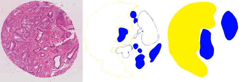
This publication of the annotations also unfortunately reveals the potential impact of actual mistakes in these annotations. About 15% of the annotations in the publicly released training set have an issue with unclosed borders in the manual annotations leading to an incorrect annotation map [7], as illustrated in Fig. 5. This kind of error doesn’t really fall into the category of “inter-expert disagreement", or of the expected uncertainty on a manually drawn contour, as it is clearly either a software issue (accepting unclosed borders as an input) or a workflow issue (not checking the validity of the manual annotation maps). Furthermore, it is possible that the same problem is also present in the (unpublished) annotations of the test set. This issue may call into question the accuracy of the participants’ leaderboard and lead to difficulties in comparing results from the challenge and from post-challenge publications. While the errors have been noted by some, with the removal of the mistaken annotations from the training dataset [63], many recent works using this dataset do not seem to take these mistakes into account [64]–[67].
The results reported on the challenge’s website include a ranking of all the teams based on a custom score which combines the Cohen’s kappa and the F1 score, as well as a confusion matrix of the pixel grading for each of the top 8 teams, normalised so that each row (representing the “ground truth" grade) sums up to 1, providing the sensitivity of each grade on the diagonal. There is no available evaluation code, and the exact definition of the metric is unclear (Cohen’s kappa could be unweighted or weighted in different ways, and the F1 score could be computed on the image-level classification task or on the pixel-level segmentation task).
The reporting of the confusion matrix, however, brings a lot of interesting information that is not apparent in the overall score (see Table 6). For instance, while the winning team is very good at classifying benign tissue (95.94% sensitivity) and much better than all other teams at classifying grade 5 tissue (73.76%, with the next team at 24.54%), it is among the worst at grade 3 (2.24%) and 4 (16.49%). It also puts into question the accuracy of the evaluation process, as there are several inconsistencies in the confusion matrices, with some rows summing up to values superior to 1 (for instance, Grade 4 of #3 sums up to 135.7%), or inferior (for instance, Grade 5 of #5 sums up to 28.29%). This could just be an error in the copying of the results to the challenge’s web page. However, if the confusion matrices were used to compute the F1 scores, this may also affect the final scores of the challenge.
| Team | Score | Benign | Grade 3 | Grade 4 | Grade 5 |
|---|---|---|---|---|---|
| #1 | 0.845 (1) | 95.94% (1) | 2.24% (8) | 16.49% (8) | 73.76% (1) |
| #2 | 0.793 (2) | 82.95% (6) | 52.73% (5) | 53.97% (4) | 24.55% (2) |
| #3 | 0.790 (3) | 90.96% (3) | 70.72% (1) | 38.69% (7) | 24.10% (4) |
| #4 | 0.778 (4) | 88.32% (5) | 66.57% (3) | 46.93% (5) | 22.90% (5) |
| #5 | 0.760 (5) | 88.96% (4) | 50.08% (6) | 70.61% (1) | 0% (6) |
| #6 | 0.758 (6) | 72.47% (8) | 67.17% (2) | 43.77% (6) | 24.54% (3) |
| #7 | 0.716 (7) | 82.89% (7) | 55.22% (4) | 63.65% (2) | 0% (6) |
| #8 | 0.713 (8) | 94.23% (2) | 37.01% (7) | 54.10% (3) | 0% (6) |
With the availability of the individual expert annotations, the challenge may also have missed the opportunity of a finer analysis of the results of the algorithms, in relation to the actual application of Gleason grading. The metrics were computed based on the STAPLE consensus, but did not look at how the algorithms compare to individual experts. As we show in a previous work [7], the available expert annotations show that some experts share very similar annotations and can be grouped into “clusters". As not all experts annotated all images, the STAPLE consensus can therefore depend on which particular experts annotations are available for a particular image. This may also influence the results, if some algorithms tend to follow some experts more than others. Comparing the algorithms to every expert at once and using visualisation techniques, such as Multi-Dimensional Scaling (MDS), could bring a better understanding of the behaviour of the algorithms than what is apparent from the results computed on the STAPLE consensus [7].
MoNuSAC 2020 has provided a level of transparency that is above what can usually be found in digital pathology challenges. The organisers publicly released the full training and test set annotations, the evaluation code, and the predictions of the top 5 teams on the test set. This kind of transparency is to be welcomed as it should make it possible to replicate the table of results from the challenge and therefore to verify the accuracy of the final rankings. Another important advantage is that the published predictions also allow researchers to calculate other metrics to enrich the evaluation and possibly extract new information from the challenge. Thus, in a recent study, we show that the use by the challenge of a metric like the Panoptic Quality, which merges together segmentation and detection metrics, can lead to a loss of relevant information that independent and simpler metrics provide [18].
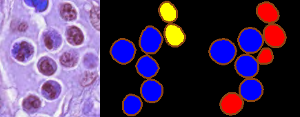
Unfortunately, there are two problems with the released top teams predictions. The first is that the link on the website for the top-ranked team is incorrect, reducing access to “#2-#5" only : still the case as of today. --AF . The second is that the released predictions are not the raw prediction maps sent by the participants and used in the evaluation, but are “colour-coded" images provided “for illustrative purposes" only, as we can see in Fig. 6. This is still a major improvement in transparency compared to most challenges.
The transparency adopted in this challenge also allowed the detection of a bigger problem, consisting of errors in the evaluation code, as we reported in our comment to the challenge article [68]. While the errors themselves are unfortunate, the fact that they could be found and corrected is entirely due to the transparency offered by the challenge organisers. It shows how important this transparency is: if similar mistakes occur in other challenges, there is absolutely no way to detect them without the publication of the predictions, the ground truth annotations and the evaluation code : obviously leaving room for others to find such mistakes is a bit scary, but this improves the trustworthiness of results so much that releasing all the code & data necessary for replication should really have become the standard by now. --AF .
Segmentation challenges require a lot of time and effort to organise. Ground-truth annotations are time-consuming and require the participation of trained experts. Meanwhile, dozens of competing teams develop and train deep learning models to solve the proposed tasks. The organisers then have to evaluate the predictions provided by each participant. The benefits of these challenges to the research community are clear: challenges offer a way to benchmark algorithms in a controlled environment. They incentivize the machine learning and computer vision research community to work on problems that are supposed to be relevant to pathologists, with possible improvements in this regard [3]. Our review of the best ranked methods show that, in terms of deep neural networks, there is a certain convergence towards “U-Net like" models with many different variants in the encoder and in the smaller details of the architecture. Most of the difference between methods, however, seem to be found in the pre- and post-processing steps. It is apparent that, in digital pathology tasks, deep neural networks cannot be used as an “end-to-end" method, and that they are generally integrated in some larger pipeline. Digital pathology images, even when not using WSIs, are usually too large to be used directly in the network. Therefore, some tiling and stitching mechanisms have to be applied. Digital pathology tasks are often also complex and can be divided into different subtasks. This is generally treated either as parallel paths in the networks or with cascading methods. Post-processing steps often include some domain-specific knowledge to filter the raw results of the models and ensure that results that are highly improbable are filtered out.
All these insights are valuable information that are made more apparent thanks to the organisation of challenges. While our analysis of the segmentation challenges does not take away from these benefits, they do highlight some important points of attention that severely limit their current value.
There is currently a significant gap between the recognized importance of inter-expert agreement in digital pathology, which is regularly mentioned in reviews [2], [3], [11] and/or measured in challenge publications [19], [27], [31], and its inclusion in the evaluation of the challenge itself. Most challenges either rely on a single expert or on an informal consensus of several experts whose individual opinions are not recorded. Gleason 2019 is the only exception to this trend. Yet, when the inter-expert agreement is measured, it is clear that the differences between algorithms according to the evaluation metrics are often smaller, or of the same order, as the differences between experts. The resulting ranking of the algorithms will therefore be very sensitive to the particular set of experts that were involved in the consensus for each particular image, as demonstrated by [2].
To solve this problem, it is important that challenges take care of documenting the inter-expert agreement, not only as a separate measure from the challenge ranking and used in the discussion to contextualise the results, but also as a property of the dataset itself. This consideration opens up different possibilities in the evaluation process and the discussion, such as:
Comparing the algorithm and expert agreement to the “consensus" at the level of the individual images (e.g., checking whether the algorithms tend to disagree with each other on the same images as the experts).
Better measuring whether an algorithm is truly “better" than another, or whether both are within the range of expert agreement.
Making sure that the rankings are robust to the particular selection of experts, for instance by computing the results for different subsets of experts.
Most digital pathology segmentation challenges use some variations of the DSC, IoU and/or HD metrics. There are, however, many different choices in the implementation of the metrics, such as task-specific adaptation, or in the aggregation process. The complexity of digital pathology tasks make it very difficult to have a single metric that covers all the important aspects of the evaluation. When such an overarching metric is used, it inevitably compresses the information that can be inferred from it about the performance of the algorithms. Combining independent metrics into a single ranking is also very difficult. In all cases, there are some arbitrary choices that need to be made, and the influence of those choices in the ranking is difficult to separate from the actual performance of the algorithms.
There seems to be a conflict between the scientific objectives of the challenges (gaining insights on the performance of algorithms) and their competitive objectives (announcing a winner). A practical solution to this conflict would be to increase transparency on the results. If the raw predictions of the challenge participants and the test set annotations are available to researchers after the challenge, interested parties can compute additional metrics and perform further analysis of the results, to gain more insights on some aspects of the task that may not have been properly captured in the original ranking.
To fully understand the published results, it is also important that the evaluation method be precisely described by the organisers. Unfortunately, this is not always the case. The use of a standardised challenge description, such as the BIAS report used for MICCAI challenges [69], is a good step forward, provided that this report is public and easy to find. For instance, the BIAS report of the PAIP 2021 challenge is available on Zenodo, but without a link to it on the challenge website.
Even when the evaluation method is well described, some choices are really made at the implementation level. To have the full picture of how the methods are evaluated, it is therefore necessary for the evaluation code to be public.
As already mentioned, the organisation of digital pathology challenges is a very complex process that is inevitably subject to errors. These errors can happen anywhere from the annotation process to the evaluation code or the analysis of the results. They can also significantly impact the results of the challenge, and therefore the conclusions drawn from them, influencing the trends in designing models and algorithms to solve similar tasks in the future.
There is therefore a large responsibility that is shared by the challenge organisers, the participants, and the research community that uses the datasets and the results of the challenges afterwards, to be vigilant and to actively participate in the quality control of the challenges. For challenge organisers, being as transparent as possible, by providing participants and future researchers with the means to replicate the results of the challenge, ensures better quality control. This passes through the public release of the evaluation code, the test set annotations, and the participants’ predictions. It is then also the responsibility of the challenge participants to check that the results are correct and to contribute to their analysis. So, for example, regarding the errors in the MoNuSAC 2020 challenge evaluation code, the responsibility for not finding these errors in time is shared with the participants since the code is publicly available since the start of the challenge.
Computer vision in digital pathology has come a long way since the ICPR 2010 challenge. The move from “classic" computer vision algorithms to deep convolutional neural networks, and the evolution of those networks, can be followed through the results of the challenges. Many of the popular network architectures of the past and present, such as AlexNet [70], Inception [71] or U-Net [45] first demonstrated their capabilities in computer vision challenges.
Segmentation challenges in digital pathology are extremely difficult to organise and to properly evaluate. The complexity of the underlying pathology tasks and the uncertainty on the ground truth, due to interexpert disagreement and the difficulty of creating precise annotations in a reasonable amount of time, contribute to these difficulties.
It is therefore important to ensure that these challenges are designed to be as useful as possible to the research community, beyond the competition itself. The rankings and prize-giving are very useful in getting the larger computer vision and deep learning community involved in digital pathology tasks. However, we need to ensure that the competitive aspects do not detract from the insights that we seek to establish.
The largest obstacle to being able to fully leverage the potential of challenges appears to be insufficient transparency. Restricting access to the datasets (and the test dataset in particular) is obviously necessary while the challenge is underway, but becomes a barrier to subsequent research once the challenge is over. Challenge websites are also often abandoned once the final ranking has been published and/or the related conference event is over. Even though all the reviewed challenges are relatively recent, a lot of the information has been lost, or has become very difficult to find, with some websites no longer available, some links to the datasets no longer working, and contact email addresses not responding as organisers have moved on to other projects.
Having access to the evaluation code, the participants’ predictions and the full dataset, including the test set annotations, is the only way to ensure that the results are reproducible and can be properly compared to new results provided by other methods. In turn, this comparison can be freed from the choices that the challenge organisers have made in the evaluation process, and be based on other measures that might be more relevant.
Digital pathology challenges are already very valuable to the research community. Improving their transparency could increase their value, and help to transition from the competitive process of the challenge itself to the more collaborative nature of the post-challenge research, where researchers can improve and learn from each other instead of working independently and comparing their results after the fact. This would allow their potential to be fully exploited.
The CMMI is supported by the European Regional Development Fund and the Walloon Region (Wallonia-biomed; grant no. 411132-957270; project “CMMI-ULB”). CD is a senior research associate with the Fonds National de la Recherche Scientifique (Brussels, Belgium). CD and OD are active members of the TRAIL Institute (Trusted AI Labs, https://trail.ac, Fédération Wallonie-Bruxelles, Belgium).
Adrien.Foucart@ulb.be↩︎
https://warwick.ac.uk/fac/cross_fac/tia/data/glascontest/evaluation/↩︎