---- 4.1 Definitions
------ 4.1.1 Evaluation process
------ 4.1.2 Detection metrics
------ 4.1.3 Classification metrics
------ 4.1.4 Segmentation metrics
------ 4.1.5 Metrics for combined tasks
------ 4.1.6 Aggregation methods
---- 4.2 Metrics in digital pathology challenges
------ 4.2.1 Detection tasks
------ 4.2.2 Classification challenges
------ 4.2.3 Segmentation challenges
---- 4.3 State-of-the-art of the analyses of metrics
------ 4.3.1 Relations between classification and detection metrics
------ 4.3.2 Interpretation and problems of Cohen's kappa
------ 4.3.3 Imbalanced datasets in classification tasks
------ 4.3.4 Statistical tests
---- 4.4 Experiments and original analyses
------ 4.4.1 Foreground-background imbalance in detection metrics
------ 4.4.2 Imbalanced datasets in classification tasks
------ 4.4.3 Limit between detection and classification
------ 4.4.4 Use of detection metrics for instance classification
------ 4.4.5 Agreement between classification metrics
------ 4.4.6 Biases of segmentation metrics
------ 4.4.7 Multi-metrics aggregation: study of the GlaS 2015 results
------ 4.4.8 Why panoptic quality should be avoided for nuclei instance segmentation and classification
---- 4.5 Recommendations for the evaluation digital pathology image analysis tasks
------ 4.5.1 Choice of metric(s)
------ 4.5.2 Using simulations to provide context for the results
------ 4.5.3 Disentangled metrics
------ 4.5.4 Statistical testing
------ 4.5.5 Alternatives to ranking
---- 4.6 Conclusion
4. Evaluation metrics and processes
In challenges or in any publication that aims to determine if a particular method improves on the state-of-the-art for a particular task, the question of how to evaluate the methods is extremely important. At the core of any evaluation process, there is one or several evaluation metrics. Different metrics have been proposed and have achieved a more-or-less standard status for all types of tasks, and many studies have been made to examine their behaviour in different circumstances. Moreover, the evaluation process is not limited to the metric itself.
In this chapter, we will start in section 4.1 by providing the necessary definitions for the description of the evaluation process of digital pathology image analysis tasks, and of the common (and less common) evaluation metrics used for detection, classification, and segmentation tasks, as well as for more complex tasks that combine these different aspects. The use of these metrics in digital pathology challenges will then be discussed in section 4.2, and the state-of-the-art of the analysis of their biases and limitations in section 4.3.
We will then present our additional analyses and experiments in section 4.4, and provide recommendations on the choices that can be made when determining the evaluation process for a digital pathology task in section 4.5.
4.1 Definitions
Most of the formal definitions of the metrics used in this section are adapted from several publications and reworked to use the same mathematical conventions. For the detection metrics, we largely rely on the works of Padilla et al. [38], [39]. Most of the classification metrics can be found in Luque et al. [32], while the definitions for the segmentation metrics are given in Reinke et al. [40]. The evaluation process in general described here is largely based on our analysis of the processes described in all the digital pathology challenges referenced in section 4.2.
4.1.1 Evaluation process
The evaluation of an algorithm in an image analysis task starts from a set of “target” samples (usually from expert annotations and considered to be the “ground truth”), associated to a set of predictions from the algorithm. In the final evaluation of an algorithm, the samples would come from the “test set” extracted from the overall dataset, which should be as independent as possible from the training and validation set. The exact nature of the samples will depend on the task.
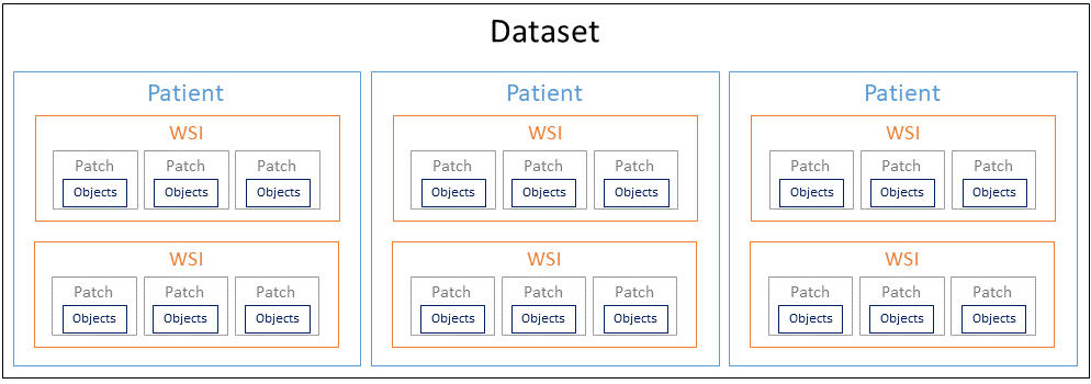
Digital pathology datasets have a hierarchical nature, with the top-level being the patient. From each patient, different whole-slide images (WSI) may have been acquired. From each of those WSIs, different image patches may have been extracted, and often each of these patches will contain a set of individual objects of interest (as illustrated in Figure 4.1).
In the DigestPath 2019 challenge1, for instance, two different datasets are described. The “signet ring cell dataset” contains objects (the signet ring cell) in 2000x2000px image patches extracted from WSIs of H&E stained slides of individual patients. In the “colonoscopy tissue segment dataset,” however, WSIs have been directly annotated at the pixel-level, so there are no “patch-level” or “object-level” items.
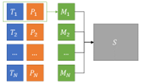
A metric is thus defined as a function that evaluates a pair of “target” (ground truth) and “predicted” items (e.g. object localization, patient diagnostic class…). Most metrics will produce outputs either in the or the range, but there are exceptions (such as distance-based metrics, which are typically in ). The aggregation process, on the other hand, describes how the set of metric values at a given level is reduced to a single score at a higher level (see Figure 4.2).
With these definitions in mind, we can now turn our attention to the three main “task types” that we previously identified in Chapter 1, as well as their combinations.
In a detection task, there will typically be an object-level annotation. To evaluate such a task, the first step is therefore to find the matching pairs of objects in the images. The matching criteria are therefore an important factor in the evaluation process. They typically involve a matching threshold, for instance based on the centroid distance or the surface overlap. Once the matching pairs of objects have been found, there are two separate aspects of the results that can be evaluated. First, a partial confusion matrix can be built:
With TP the “True Positives” (number of matching pairs), FN the “False Negatives” (number of un-matched ground truth objects), FP the “False Positives” (number of un-matched predicted objects), and is the cardinality of a set. It should be noted that, at the object-level, there are no countable “True Negatives,” which will limit the available metrics for evaluating the detection score [38].
The other possible aspect of the evaluation is the quality of the matches. This can take different forms depending on what exactly the target output was: bounding box overlap, centroid distance, etc.
In a classification task, the annotation could be at the object level (instance classification), at the pixel level (semantic segmentation), at both levels (instance segmentation and classification), or at any of the “higher” levels in Figure 4.1: patch, WSI, or even patient. The latter cases correspond to “pure” classification tasks, whereas the others are combining classification with detection and/or segmentation. The classification part of the problem can typically be summed up with a confusion matrix, built from pairs of where and is the number of classes in the problem, and with a vector of class probabilities so that . The confusion matrix will therefore be a matrix with .
The distinction between “classification” tasks and “detection” tasks can sometimes be difficult to make. In many digital pathology applications, there will be one “meaningful” class (for instance: nuclei, tumour, etc.), and a “no class” category that includes “all the rest.” In those cases, there will be clear “positive” and “negative” categories, and the confusion matrix will include the TP, FP, FN (and, in this case, countable TNs) of the detection tasks. As we will see further in this chapter, this can be a source of confusion in the definition of the metrics, as some metrics, such as the F1-Score, take a different form if a single “positive” class is considered (as in a detection task) or if two or more classes are considered on equal grounds.
The combination of “detection” and “classification” is instance classification, which can also be seen as multi-class detection. In such problems, the results can be described in a confusion matrix that includes multiple classes and a background or no-instance category. The confusion matrix for an m-class problem would therefore look like:
Where the first line corresponds to falsely positive detections (i.e. detections for any of the classes that correspond to no ground truth object) and the first column to falsely negative detections (i.e. ground truth objects that have no predictions). As in the previously described detection confusion matrix, the top-left corner is uncountable and corresponds to the true negative detections.
In segmentation tasks, the annotations will be at the pixel-level. These annotations can be simply binary (an “annotation mask”), or also contain class labels (“class map”) and/or instance labels (“instance map”). We will therefore have and , with the pixel position. In an instance segmentation case, there will once again need to be a matching criterion to find the matching subsets and , so that the evaluation can be reduced to several binary “object-level” annotation masks. In semantic segmentation, there is no matching step necessary. Instead, a segmentation metric will often simply be computed per-class, then an average score can be computed. The most common evaluation metrics can be defined from pixel-level confusion matrices, or as distance metrics that compare the contours and/or the centroids of the binary masks.
When all three tasks are combined together, we get instance segmentation and classification. In such problems, each pixel can be associated both to a class and to an instance label. The evaluation of such problems can be quite difficult, as will be discussed through this chapter.
4.1.2 Detection metrics
As mentioned above, detection tasks typically require a matching step before the evaluation, often involving a matching threshold . The matching step takes the sets of Target objects and Predicted objects and outputs three sets: the true positives, the un-matched false negatives, and the un-matched false positives.
These sets are related to a confidence threshold on the detection probability (which is the raw output of the detection algorithm), that determines if a candidate region is considered as a detected object or not: , with the detection probability for the object [38], with usually set to 0.5.
Higher confidence thresholds will yield a smaller set of , which means that the following relationships are always verified:
Detection metrics will therefore be either “fixed-threshold” metrics, bound to a particular choice for the matching and confidence thresholds, or “varying-threshold,” capturing the evolution of the metric as the thresholds are moved.
4.1.2.1 Object Matching
In most cases, object detection outputs include some sort of localisation, which gives an indication of where is the object in the image, and what is its size. In the most precise case, we have the full segmentation of the object, and are therefore in an “instance segmentation” problem. More often, the localisation will be given in the form of a bounding box with a centroid. In the extreme opposite case, there is no localisation at all, and simply an indication of whether an object is present in the image or not. There is then no “matching” step, and the problem is formulated as a binary classification problem, with the “no object” and “object” class being determined at the image patch level.
The matching step generally is “overlap-based” and/or “distance-based.”
Given a pair of target and predicted objects and , represented as a set of pixels belonging to this object (which may come either from bounding boxes or per-pixel instance masks), overlap-based methods will look at the intersection area () and the union area () of the two objects. These two measures can be combined in the intersection over union (IoU), also known as the Jaccard Index [24]:
A common criterion is to apply a threshold on this IoU, so that a pair of objects is “a match” if , with often set at 0.5 or 0.75 [39]. If , it is possible for multiple target objects to be matched to the same predicted objects (and vice-versa), in which case a “maximum IoU” criterion is typically added to the rule (so that the match is the predicted object with the maximum IoU among those that satisfy the threshold condition). In that case, we will therefore have: where all three following conditions are respected:
The maximum IoU can also be used as a single criterion, with no threshold attached, in which case any overlap may be detected as a match (this is equivalent to setting ).
Another strategy to determine a match relates to the distance between the centroids of the objects. Similarly to the IoU criterion, this will imply a “closest distance” rule, which may be associated with a “maximum distance threshold.” The criteria will therefore be:
With usually defined as the Euclidian distance between the centroids of and .
The same rule can be adapted to other distance definitions, such as for instance the Hausdorff’s distance (defined in the segmentation metrics below) between the contours of the objects.
4.1.2.2 Fixed-threshold metrics
Fixed-threshold metrics are computed for a specific value of the matching threshold (commonly, ) and of the confidence threshold (also usually ), which determine the sets TP, FP and FN.
The precision (PRE) of the detection algorithm is the proportion of “positive detections” that are correct, and is defined as:
The recall (REC) is the proportion of “positive target” that have been correctly predicted, and is defined as:
The F1-score (F1) is the harmonic mean of the two:
4.1.2.3 Varying-threshold metrics
To better characterize the robustness of an algorithm’s prediction, it is sometimes useful to look at how the performance evolves with different values of the confidence and/or matching thresholds.
Decreasing the confidence threshold means being less restrictive on what’s considered a “prediction,” and therefore to more true positives, more false positives and less false negatives. There is thus a monotonic relationship between the confidence threshold and the recall. The relationship between the precision and the confidence threshold, however, is less predictable.
This dynamic relationship between PRE, REC and the confidence threshold can be captured in a “precision-recall curve” (PR curve). An example of a PR curve is shown in Figure 4.3, constructed from synthetic data. As we can see, while the overall trend is for the precision to decrease as the recall increases, the relationship is not monotonic, and the precision has a characteristic “zig-zag” pattern.
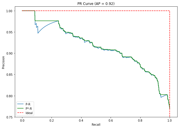
To summarize the performance shown by the PR curve, the “area under the PR curve” (AUPRC) can be computed. An ideal detector would have . A very common approximation of the AUPRC, that is less sensitive to the small oscillations of the precision, is the “Average Precision” (AP). Adapting the formulation from Luque et al. [39], we can express the PR curve as a function , and the AP is obtained by:
- Interpolating the PR curve so that , thus removing the zigzag pattern by replacing each point by the “highest value to its right” (see green line in Figure 4.3).
- Sampling with equally spaced recall values, so that
The AP is therefore a varying-threshold metric for the confidence threshold, but a fixed-threshold metric for the matching rule. To also take into account this matching rule variability, the AP can be averaged over different matching threshold values. As an example, in the NuCLS 2021 challenge [3], one of the metrics used to evaluate the detection score is the mean AP using an IoU threshold varying between 0.5 and 0.95, by step of 0.05. If we set to mean the AP using the matches found with , then we have:
4.1.3 Classification metrics
The results of a classification problem with categories are summarized in a confusion matrix. We will use here the convention that the rows of that matrix correspond to the “ground truth” class, while the columns correspond to the “predicted” class, and corresponds to the number of examples with “true class” and “predicted class” . It should be noted, however, that some of the classification metrics may be used to simply characterize the agreement between two sets of observations, without one being assumed to be the “truth.” To be useful for that latter purpose, a metric needs to be observer invariant. Practically, this is the case if (or, from the sets of ground truth and predicted observations : ).
Another characteristic of classification metrics is that they can be class-specific or global. A class-specific metric will evaluate class as a “positive” class against all others, while global metrics aggregate the class-specific values.
Metrics can also assume an order to the classes or, on the contrary, that they are purely categorical. In the former case, switching the classes in the confusion matrix would lead to a different result, while categorical metrics are class-switch invariant.
Finally, another aspect (that we more thoroughly examine in sections 4.3 and 4.4) is the class imbalance bias that many metrics exhibit. This means that changing the class balance of the dataset (e.g. by changing the sampling method) alters the results.
4.1.3.1 Class-specific metrics
Several per-class metrics can be defined. These use the notions of the True Positives (TP), True Negatives (TN), False Positives (FP) and False Negatives (FN). Using our general notation for the confusion matrix, we can have for class :
An example on a 5 classes problem is shown in Table 4.1.
| T \ P | |||||
|---|---|---|---|---|---|
The sensitivity (SEN), also called recall (REC) or True Positive Rate (TPR) measures the proportion of “True Positives” among all the samples that are “positive” in the Target (i.e. that truly belong to the class ):
The specificity (SPE), or True Negative Rate (TNR) is conversely the proportion of TN in the negative Target samples:
The precision (PRE) or Positive Predictive Value (PPV) is the proportion of TP in the positive Predicted samples:
The Negative Predictive Value (NPV) is similarly the proportion of TN in the negative Predicted samples:
The False Positive Rate (FPR) is the proportion of FP in the negative Target samples:
The F1-Score is better defined as a detection metric (see section 4.1.2), but it is often used in classification problems as well.
The per-class F1-Score () is defined as the harmonic mean of the precision and sensitivity:
The per-class Geometric Mean () of the SEN and SPE is also sometimes used [32]:
4.1.3.2 Global metrics
To get a global classification score that aggregates the results from all classes, several metrics are possible.
The simplest performance measure from the confusion matrix is the accuracy (ACC), which is given by the sum of the elements on the diagonal (the “correct” samples) divided by the total number of samples :
It is also possible to extend the F1-Score so that it becomes a global metric. The macro-averaged F1-Score has been defined in two different ways in the literature [42].
First, as a simple average of the per-class F1-scores. We call this version the simple-averaged F1-Score ():
The other definition first computes the average of the per-class PRE and SEN, before computing the harmonic mean. We will call it the harmonic-averaged F1-Score ():
With:
Meanwhile, the micro-averaged F1-Score () will first aggregate the TP, FP and FN before computing the micro-precision and micro-recall, and finally the F1-Score. It has been used in challenges such as Gleason 2019, but it should be noted that it is equivalent to the accuracy:
Like the F1-Score, the can also be extended as a global metric. It will then be the Geometric Mean (GM) of the per-class :
The GM has zero bias due to class imbalance [32]. It is, however, not observer invariant.
The Matthews Correlation Coefficient (MCC), often called in the multiclass case (and sometimes phi coefficient), uses all the terms of the CM and is defined as:
It is bound between -1 and 1, where 0 means that the target and prediction sets are completely uncorrelated.
Cohen’s kappa is a measure of the agreement between two sets of observations and can be used as a classification metrics to rate the agreement between the target and the predictions. It measures the difference between the observed agreement and the agreement expected by chance , and is defined as [8]:
So that a “perfect agreement” () leads to , a perfect disagreement () to a negative (the exact minimum value depends on the distribution of the data). From the confusion matrix, and are defined as:
Cohen’s kappa is also often used for ordered categories, where errors between classes which are “close” together are less penalised.
Let be a weight matrix ( should verify , and ).
We can define the matrix of expected observations from random chance with:
From that, we define Cohen’s kappa generally with:
The three most common formulations of the weights are:
Unweighted kappa : (using the Kronecker delta), which resolves to the same value as the original definition of the shown above.
Linear weighted kappa :
Quadratic weighted kappa :
Cohen’s kappa is bound between -1 and 1, with 0 corresponding to as much agreement as expected by random chance.
4.1.3.3 Varying-threshold metrics
All the classification metrics described thus far are “no threshold” metrics, where the predicted class of a sample is simply taken as the class which has the maximum predicted probability. It can however also be interesting to take into account the “confidence” of a model with regards to its predictions. This information can be captured in a “Receiver Operating Characterstic,” or ROC Curve. Where the detection PR-curve plotted the PRE and REC for varying confidence thresholds, the ROC curve plots the SEN (=REC) and the FPR (=1-SPE).
As the SEN and SPE are “per-class” metrics, so is the ROC a “per-class” visualisation, where the “varying threshold” is used in a “one class vs all” manner. For a class , a threshold , and the set of predicted class probabilities vectors where is the probability that sample has the class , we can define:
From which and can be computed.
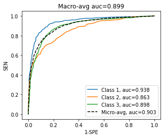
To summarize the information contained in the ROC curve, the Area Under the ROC () can be computed for a class, so that an “ideal classifier” for that class would have an of 1. As for the F1-Score, we can also define micro-averaged and macro-averaged summaries of the .
The macro-average is defined as:
While the micro-averaged is defined by first summing the TP, FP, TN and FN:
, etc.
Then computing the resulting , , and finally the from those micro-averaged values. An example on synthetic data is presented in Figure 4.4.
A summary of the main characteristics of the metrics discussed here can be found in Table 4.2.
| Metric | Range of values | Class-specific or global | Observer invariant | Class imbalance bias | Ordered |
|---|---|---|---|---|---|
| [0, 1] | Class-specific | No | No | No | |
| [0, 1] | Class-specific | No | No | No | |
| [0, 1] | Class-specific | No | High | No | |
| [0, 1] | Class-specific | No | High | No | |
| [0, 1] | Class-specific | Yes | High | No | |
| [0, 1] | Class-specific | No | No | No | |
| [0, 1] | Global | Yes | Medium | No | |
| [0, 1] | Global | Yes | Low | No | |
| [0, 1] | Global | Yes | Medium | No | |
| [-1, 1] | Global | Yes | Medium | No | |
| [-1, 1] | Global | Yes | High | No | |
| [-1, 1] | Global | Yes | High | Yes | |
| [0, 1] | Global | No | No | No | |
| [0, 1] | Class-specific | No | No | No | |
| [0, 1] | Global | No | No | No | |
| [0, 1] | Global | No | No | No |
4.1.4 Segmentation metrics
We consider in this section pure “segmentation” tasks that separate a foreground region from a background region. Instance and semantic segmentation will be considered in the “combined metrics” section. Segmentation metrics therefore compare two binary masks in an image. Let be the set of pixels that belong to the target (“ground truth”) mask, and the set of pixels that belong to the predicted mask. There are two main categories of segmentation metrics: those that measure the overlap between the two sets, and those that measure a distance between the contours of the and masks, labelled and respectively.
In the following definitions, is the cardinality of the set and indicates all the elements that are not in the set.
4.1.4.1 Overlap metrics
The overlap metrics can also be defined using a “confusion matrix” based on the binary segmentation masks and (we use here boldface to denote the mask matrices instead of the sets), where for all , otherwise. The TP, FP, FN and TN are then defined as:
The two most commonly used overlap metrics are the Dice Similarity Coefficient (DSC) and the Intersection over Union (IoU), while the most common distance-based metric is Hausdorff’s Distance (HD). The IoU, DSC and HD are illustrated in Figure 4.5.
![Figure 4.5. Illustration of the three “basic” segmentation metrics. Adapted from our review [15].](./fig/4-5.png)
The IoU is defined as:
It is bounded between 0 (no overlap) and 1 (perfect overlap).
Using the confusion matrix notation, it can also be defined as:
The DSC is defined as:
It is also bounded between 0 and 1, and heavily correlated to the IoU, as the two are linked by the relationship:
That relationship also means that is always verified.
Like the IoU, we can define it in terms of the confusion matrix values:
Which shows that it simply corresponds to a “per-pixel” definition of the F1-score.
4.1.4.2 Distance metrics
For Hausdorff’’s distance (HD), only the contours and are considered. First, the Euclidean distances from all points in to the closest point in are computed, and the maximum value is taken:
Then, the same thing is done starting from all the points in :
Hausdorff’s distance is then defined as the maximum of those two values:
This process is illustrated in Figure 4.6.
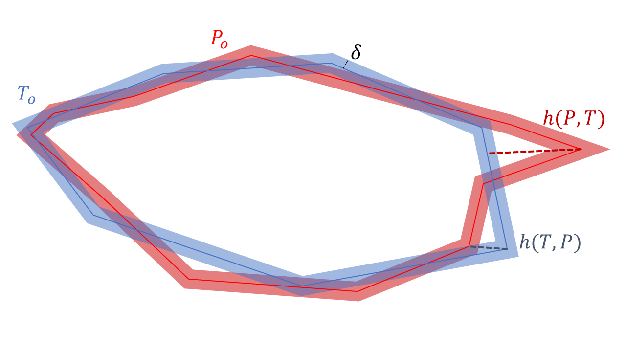
As the HD is extremely sensitive to outliers, it is also sometimes preferred to slightly relax the “maximum,” and to replace it with a percentile :
With being the most frequent choice.
While a HD of 0 corresponds to a perfect segmentation, its maximum value is unbounded. This makes it a particularly tricky metric to use in aggregates, as it is difficult to assign a value, for instance, to a “missing prediction” (i.e. an image where ).
While less commonly used, some other distance-based metrics exist. Reinke et al.’s review [40] notably mention the Average Symmetric Surface Distance (ASSD) and the Normalized Surface Distance (NSD).
The ASSD is defined as:
For each point of the contour, the distance to the other contour is computed. The final value is the average distance computed from both contours. Compared to the HD, it will tend to penalize more a segmentation that is consistently wrong by a small amount than a segmentation that is almost perfect but with a few large errors.
The NSD, meanwhile, is a metric that takes into account the uncertainty of the annotations by first defining “boundary regions” and , which are the set of all pixels within a certain tolerance distance of the contours and :
The NSD is then defined as:
This same idea of a “tolerance” could easily be applied to the HD as well by redefining the and as:
So that the “uncertainty-aware” is given by:
4.1.4.3 Segmentation as binary classification
The IoU and DSC metrics, in their “confusion matrix” definitions, are essentially “pixel detection” metrics, which do not take into account the “true negatives” and consider that there is a “positive” class, the foreground, and a “negative” class, the background. But once we have established the confusion matrix, it is also possible to treat the problem as a “binary classification” problem, including the true negatives. The classification metrics defined in 4.1.3 can therefore also be used. The ACC or the MCC, for instance, can easily be computed.
The main difference of this approach is that it does not consider that the “foreground class” is inherently more important than the “background class,” and that the metric should reflect that correctly identifying that a pixel is in the background is just as important as identifying one in the foreground.
A key benefit is that it becomes trivial to extend the metrics to the semantic segmentation case, as adding new classes just means adding new rows and columns to the confusion matrix, but the formula for computing the metrics remains unchanged.
The main drawback of this approach is that, when the segmentation metric is computed on patches extracted from a larger image (for instance, comparing just the masks of a detected object and its matching ground truth object), the result of the metrics becomes highly dependent on the size of the patches, and the amount of background included in it.
Binary segmentation problems are indeed typically not really “two classes” problems, but rather “one class” class problems where we detect one class and put all others in the same bin. The “per-pixel binary classification” approach would therefore only make sense if the problem can actually be defined as a two classes problem.
4.1.5 Metrics for combined tasks
The most common approach for the evaluation of combined tasks (instance segmentation, semantic segmentation, instance classification, instance segmentation and classification) is to combine “basic” metrics to create a new one which attempts to summarize all aspects of the task into a single score.
The Gleason 2019 challenge, for instance, combines a classification with a micro-averaged and a macro-averaged segmentation F1-Score into a score . The SNI challenges, meanwhile, combine a simple “binary” DSC (on the whole image and not on separate instances) with a sort of micro-averaged DSC where the numerator and denominator of the DSC are separately aggregated over the set of matching instances. A similar idea is used in the MoNuSeg challenge with the “Aggregated Jaccard Index” (AJI), where the Intersection and the Union are aggregated over the matches.
For the most complex task of instance segmentation and classification, the “Panoptic Quality” (PQ), originally proposed by Kirillov et al. [27] for natural scenes, has recently been introduced to digital pathology by Graham et al. [20].
The PQ considers each class separately. For each class , is the set of ground truth instances in the class. Given a set of corresponding class predictions , the is computed in two steps.
First, the matches between ground truth instances and predicted instances are found (using the matching threshold). Using this strict matching rule, each segmented instance in and can be counted as TP, FP or FN.
Then, the of the class in the image is computed as:
Which can be decomposed into:
With the “Recognition Quality,” corresponding to the per-object F1-score of the class , and the “Segmentation Quality,” corresponding to the average IoU of the matching pairs of ground truth and predicted instances. The is also often referred to as the Detection Quality, and therefore noted as [43], [20].
4.1.6 Aggregation methods
A critical step to arrive at a final “score” for an algorithm on set of test samples is the aggregation of the per-sample metric(s). Let us therefore go back to the hierarchical representation of digital pathology datasets that we used at the beginning of the chapter (see Figure 4.1).
The aggregation process can happen in different dimensions: across that hierarchical representation, across multiple classes, and across multiple metrics.
4.1.6.1 Hierarchical aggregation
The aggregation across the hierarchical aggregation has two aspects: where are the metrics computed, and how are they averaged?
Object-level metrics would typically be those used in instance segmentation (per-object IoU, HD…). In a “bottom-up” approach, all the object-level measures could be averaged over a patch, then the patch-level measures over a WSI, the WSI-level over a patient, and finally the patient-level measures over the whole dataset. The problem of this approach is that, if the patches are very dissimilar in their object distribution, it may lead to cases where a single error on a patch with few objects is penalized a lot more harshly than an error on a larger patch with a larger population of objects. A more robust approach will therefore generally be to rather aggregate the per-object metrics over a WSI or a patient. It is also possible to directly average the object-level metrics on the entire dataset, skipping intermediate levels entirely. In the digital pathology context, having a patient-level distribution of a metric is however often desirable for a clinically relevant analysis of the results of an algorithm, as the goal will generally be to be able to validate that the performance of an algorithm is good across a wide range of patients. It also makes it possible to use powerful statistical tests to compare different algorithms together, as patients can then be used as paired samples.
Patch-level metrics are very commonly used in all sorts of tasks. It could be a region segmentation metric like the IoU or DSC, an object detection metric like the F1-Score, or a classification metric like the ACC or the MCC. It is once again possible to directly average those results on the entire dataset, or to go through the patient-level first.
Another possibility for many of those metrics is to not compute the metric at the patch level, but to aggregate its base components over a patient or WSI. For instance, a confusion matrix can be built over multiple patches of a WSI, before computing the relevant classification or detection metrics on this aggregated confusion matrix. This reduces the risk of introducing biases from the patch selection and focuses the results on the object of interest of pathology studies: the patient. We therefore find here again the same choices of micro- and macro-averaging that were described in the classification metrics.
4.1.6.2 Multiclass aggregation
When multiple classes are present, detection and segmentation metrics are generally first computed independently for each class before being aggregated together. This aggregation can also happen at any point in the hierarchy of the dataset. For the PQ metric, for instance, some aggregate the at the image patch level as , then find the global [43], [20], [18], while others averages each separately over all patches as , then define the global [19] (with the number of images and the number of classes). As always, the micro- or the macro-averaging approaches can also be considered. In a micro-averaging approach, the metric must first be decomposed into its base components, which are aggregated separately before computing the metric. For most classification or detection metrics, the base components would be the elements of the confusion matrix. For combined metrics such as the PQ or some custom score, then a choice must be made as to what constitutes a “base component.” Practically, almost all publications and challenges use a macro-averaging approach.
4.1.6.3 Multi-metrics aggregation
Single metrics are not capable of fully representing the capabilities of a given model or algorithm. This is true even for simple tasks: as we have seen, different metrics have distinct behaviours and biases, and may therefore miss some important insights about a particular algorithm. A clear example would be the IoU and the HD for segmentation metrics, which give very different information about the same task. As noted in section 4.1.5, combined tasks are often evaluated by creating complex metrics that combine basic detection, classification and segmentation metrics in some ways. Another approach, however, is to compute and report those simple metrics independently, to provide more detailed information about the predictive performance. Computing multiple metrics, however, means that algorithms cannot necessarily be ranked based on a single score, thus making the overall ranking (and therefore the choice of the “best method”) more difficult to obtain.
A possible solution is to compute the ranks separately for the different metrics, then to combine them with, for instance, the “sum of ranks.” As we will discuss below in section 4.4.7, this approach comes with its own pitfalls and challenges.
4.2 Metrics in digital pathology challenges
We examine here the evaluation metrics used in the challenges previously presented in Chapter 3, to get a sense of the common choices made by challenge organizers when determining the evaluation process. We look here mainly at the “basic” metrics (i.e. pure detection, classification or segmentation), and we will note when those metrics are included as part of a more complex evaluation score.
4.2.1 Detection tasks
A summary of the evaluation metrics used in digital pathology detection challenges can be found in Table 4.3. Almost all challenges used the F1-Score as the primary metric for ranking the participants’ submissions. Some challenges reported the PRE and REC separately. The only “challenge” to use varying-threshold metrics is NuCLS 2021. This dataset, however, is presented more as a benchmark for future usage by researchers than as a challenge, despite being listed on the grand-challenge.org website. In the baseline results reported by Amgad et al. [3], the AP using a fixed matching threshold of 0.5 on the IoU, and the mAP using varying matching thresholds from 0.5 to 0.95 are used, so that both the confidence threshold and the IoU threshold are varying in the metric. DigestPath ranks three different metrics separately, then use the average rank as the overall rank for each competing team.
| Challenge | Target | Metric(s) |
|---|---|---|
| PR in HIMA 2010 | Centroblasts in follicular lymphoma. | REC, SPE2 |
| MITOS 2012 | Mitosis in breast cancer. | F1, PRE, REC |
| AMIDA 2013 | Mitosis in breast cancer. | F1, PRE, REC |
| MITOS-ATYPIA 2014 | Mitosis in breast cancer. | F1, PRE, REC |
| GlaS 2015 | Prostate glands | F1 |
| TUPAC 2016 | Mitosis in breast cancer. | F1 |
| LYON 2019 | Lymphocytes in breast, colon and prostate. | F1 |
| DigestPath 2019 | Signet ring cell carcinoma. | PRE, REC, FPs per normal region, FROC3. |
| MoNuSAC 2020 | Nuclei | F1 (as part of the PQ) |
| PAIP 2021 | Perineural invasion in multiple organs. | F1 |
| NuCLS 2021 | Nuclei in different organs. | AP@.54, mAP@.5:.95 |
| MIDOG 2021 | Mitosis in breast cancer. | F1 |
| Conic 2022 | Nuclei | F1 (as part of the PQ) |
:Table 4.3. Summary of the metric(s) used in digital pathology detection challenges. Bolded values are used for the final ranking.
4.2.2 Classification challenges
A summary of the metrics used in digital pathology classification challenges is presented in Table 4.4. Compared to the detection tasks, there is a lot more diversity in the choices made by challenge organisers. All of the multi-class tasks in these challenges (except NuCLS 2021) have some form of ordering present in their categories. For the binary classification tasks, many challenges are assessed with a positive-class only metric, as shown with CAMELYON 2016 and PatchCamelyon 2019 (AUROC of the metastasis class), DigestPath 2019 (AUROC of the malignant class), HeroHE 2019 (F1-Score, AUROC, SEN and PRE of the HER2-positive class) and PAIP 2020 (F1-Score of the MSI-High class). In the multi-class case, the TUPAC 2016 and PANDA 2020 evaluations use the weighted quadratic kappa, while in MITOS-ATYPIA 2014 a “penalty” system is used for errors of more than one class. In several challenges, however, this ordering is not taken into account at all. This is the case with the Brain Tumour DP 2014, BIOIMAGING 2015 and BACH 2018 challenges, where the simple accuracy is used, and for the C-NMC 2019 challenge, where a weighted macro-averaged is preferred.
| Challenge | Classes | Metric(s) |
|---|---|---|
| Brain Tumour DP 2014 | Low Grade Glioma / Gliobastoma | ACC |
| MITOS-ATYPIA-14 | Nuclear atypia score (1-3) | ACC with penalty5 |
| BIOIMAGING15 | Normal, benign, in situ, invasive | ACC6 |
| TUPAC16 | Proliferation score (1-3) | |
| CAMELYON16 | Metastasis / No metastasis | |
| BACH18 | Normal, benign, in situ, invasive | ACC |
| C-NMC19 | Normal, malignant | Weighted sF17 |
| Gleason 2019 | Gleason grades | (included in a custom score) |
| PatchCamelyon19 | Metastasis / No metastasis | |
| DigestPath19 | Benign / Malignant | |
| HeroHE20 | HER2 positive / negative | , , , |
| PANDA20 | Gleason group (1-5) | |
| PAIP20 | MSI-High / MSI-Low | |
| NuCLS21 | Different types of nuclei |
These classification tasks make the boundaries between detection, classification and regression tasks sometimes difficult to determine. In HeroHE 2020, for instance, the ranking of the algorithm is based on the “F1-Score of the positive class,” which is a typical detection metric, but the AUROC of the positive class is also computed, which takes the “true negatives” into account and is typically a classification metric. The tasks that are explicitly about predicting a “score” all attempt to incorporate the notion of “distance” to the ground truth into their metric, which brings them closer to a regression task. The use of the quadratic kappa is also clearly related to its popularity in pathology and medical sciences in general, as it makes the results more relatable for medical experts. The danger of that particular metric, however, is that it may give a false sense of “interpretability,” as the number of classes and the target class distribution have a large effect on the perceived performance of an algorithm using that metric.
4.2.3 Segmentation challenges
Almost all segmentation challenge use overlap-based metrics (either the IoU or the DSC) as their main metric for ranking participating algorithms, as shown in Table 4.5. The only challenge to really use a distance-based metric as part of the ranking was the GlaS 2015 challenge, which ranked the per-object average HD and the per-object average DSC (as well as the detection F1 score) separately. PAIP 2021 used the HD as a matching criterion but did not use it for the ranking.
The BACH 2018 challenge is an outlier in this, as they use a custom score that loosely corresponds to a “per-pixel” accuracy, with ordered classes so that “larger” errors are penalized more.
Table 4.5. Summary of the metric(s) used in digital pathology segmentation challenges.
| Challenge | Target | Metric(s) |
|---|---|---|
| PR in HIMA 10 | Lymphocytes | DSC, IoU, HD, MAD |
| Brain Tumour DP 14 | Necrosis region | DSC |
| GlaS 2015 | Prostate glands | DSC, HD |
| SNI 15-18 | Nuclei | DSC8 |
| MoNuSeg 18 | Nuclei | IoU9 |
| BACH 18 | Benign / in situ / invasive cancer regions | Custom score |
| Gleason 19 | Gleason patterns | DSC10 (included in a custom score) |
| ACDC@LungHP 19 | Lung carcinoma | DSC |
| PAIP 19 | Tumour region | IoU |
| DigestPath 19 | Malignant glands | DSC |
| BCSS 19 | Tumour / stroma / inflammatory / necrosis / other tissue segmentation. | DSC |
| MoNuSAC 20 | Nuclei (epithelial / lymphocyte / neutrophil / macrophage) | IoU (as part of the PQ) |
| PAIP 20 | Tumour region | IoU |
| SegPC 21 | Multiple myeloma plasma cells | IoU |
| PAIP 21 | Perineural invasion | HD |
| NuCLS 21 | Nuclei (many classes) | IoU, DSC |
| WSSS4LUAD 21 | Tumour / stroma / normal tissue | IoU |
| CoNIC 22 | Nuclei (epithelial / lymphocyte / plasma / eosinophil / neutrophil / connective tissue) | IoU (as part of the PQ) |
4.3 State-of-the-art of the analyses of metrics
There is a growing amount of literature on the topic of evaluation metrics, within the context of biomedical imaging or in general. Reinke et al. [40] thoroughly examine the pitfalls and limitations of common image analysis metrics in the context of biomedical imaging. Luque et al. [32] examine the impact of class imbalance in binary classification metrics. Their methods and conclusions will be explored more deeply in section 4.3.3, and we extend their analysis in section 4.4.2. Chicco et al. [7] compare the MCC to several other binary classification metrics and find it generally more reliable. Delgado et al. [9] describes the limitations of Cohen’s kappa compared to the Matthews correlation coefficient, and some of their results are discussed below in section 4.3.2. Grandini et al [21] propose an overview of multi-class classification metrics, a topic generally less explored in the literature. Padilla et al. [38], [39] compare object detection metrics and note the importance of precisely defining the metrics used, as the AP, for instance, which can be computed in several ways.
Oksuz et al. [37] focus on object detection imbalance problems. They review the different sampling methods that can help to counteract the foreground-background imbalance to train machine learning algorithms. They identify four classes of such methods: hard sampling (where a subset of positive and negative examples with desired proportions is selected from the whole set), soft sampling (where the samples are weighted so that the background class samples contribution to the loss is diminished), sampling-free (where the architecture of the network, or the pipeline, are adapted to address the imbalance directly in the training with no particular sampling heuristic), and generative (where data augmentation is used also to correct the imbalance by increasing the minority class samples). In section 4.4.1, we also explore the effect of foreground-background imbalance on the evaluation process.
4.3.1 Relations between classification and detection metrics
Many evaluation metrics are related or take similar forms. The most obvious relationship is between the different forms of the F1-Score, which can be used as a detection measure, a classification measure, and a segmentation measure (as the DSC).
A somewhat less obvious relation exists between the F1-Score and unweighted Cohen’s kappa, as identified by Zijdenbos et al. [45]. In a binary classification where we consider a “positive” and a “negative” class, we have the confusion matrix:
And resolves to:
In a detection problem, TN is uncountable, but it can generally be assumed to verify:
With this assumption, for detection can be simplified to:
Which is the harmonic mean of the PRE and REC, i.e. the detection F1-Score.
Meanwhile, the same exercise applied to the MCC leads us to a “detection” version of:
Which is the geometric mean of the PRE and REC (note that this is different from the classification GM we used before, which was the geometric mean of the REC and SPE, not REC and PRE).
While the harmonic mean is typically the preferred averaging methods for ratios (such as the PRE and REC), the geometric mean will penalize less harshly small values for one of the averaged elements. For instance, for and , the geometric mean will still be equal to 0.3 while the harmonic mean will drop to 0.18.
4.3.2 Interpretation and problems of Cohen’s kappa
Cohen’s kappa is very popular in digital pathology. It is often associated to an “interpretation” scale such as this one [1]:
< 0: less disagreement than random chance.
0.00-0.20: slight agreement
0.21-0.40: fair agreement
0.41-0.60: moderate agreement
0.61-0.80: substantial agreement
0.81-1.00: almost perfect agreement
There is however some debate on the validity of these interpretation, with some authors suggesting that, for medical research in particular, a less optimistic view of the value should be used [34]. It should also be noted that the kappa values are highly dependent on the weights used, and that this interpretation can therefore be highly misleading if a weighted kappa is used. For instance, in McLean et al.’s study of interobserver agreement in Gleason scoring [35], looking at the unweighted kappa would lead to an interpretation of “slight agreement,” the linear kappa to “slight to fair agreement,” and the quadratic kappa to “fair to moderate agreement.”
This can be problematic when, for instance, Humphrey et al. [22] compare the average unweighted kappa of 0.435 of general pathologists on Gleason scoring from a study [2] with the 0.6-0.7 weighted kappa11 for urologic pathologists from another [1] to find an “enhanced interobserver agreement” for the specialists, instead of using the 0.47-0.64 unweighted kappa which was also reported in the same study, marking an improvement that is still very substantial but not quite as extreme as Humphrey’s paper suggests.
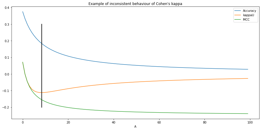
As noted by Delgado et al. [9], in some circumstances Cohen’s kappa can have an inconsistent behaviour, where a worse agreement leads to better results. In general, this can be demonstrated using the family of imbalanced confusion matrices, defined by:
So that everywhere except for , with . Intuitively, increasing means that at the same time we increase the imbalance, and we reduce the agreement. While we would expect in that case to be monotically decreasing, Delgado et al. show that it is not the case, and that after the inflexion point at the values start to increase. This can be verified experimentally, as we can see in Figure 4.7.
However, this is unlikely to happen, and in practice the in general agrees well with the MCC, as shown in our experiments in section 4.4.5.
4.3.3 Imbalanced datasets in classification tasks
The question of how classification metrics behave with imbalanced datasets was systematically explored by Luque et al. [32] for binary classification. In this section, we will briefly explain their method and their results. In section 4.4.2, we will extend their analysis to some metrics that they did not include, and to multi-class problems.
To analyse the metrics’ behaviour, the first step is to parametrize the confusion matrix so that it becomes a function of the sensitivity of each class, and of the class imbalance. Let be the sensitivity of class and the proportion of the dataset that is of class , so that and . As it is a binary classification problem, Luque et al. further define one of the classes as the positive class, and the other as the negative class. We therefore have , and we can then define the balance parameter , so that corresponds to balanced data, to an “all-negative” dataset, and to an “all-positive” dataset. The binary confusion matrix can be formulated as:
With the total number of samples in the dataset.
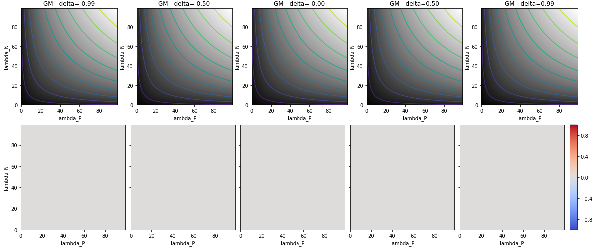
The study then shows how different classification metrics behave for different values of . The bias of a metric due to class imbalance can be characterized by looking at the difference between the metric measured for with the same metric measured at (i.e. for the same per-class sensitivities in a balanced dataset). Figure 4.8 shows for instance how the ACC behaves with imbalanced datasets. The interpretation of the top row is that, as the balance skews towards one of the two classes, only the performance of that class influences the result of the metric, as the isocontours (shown at 0.1 intervals in the figures) become parallel to either the horizontal or the vertical axis. In the bottom row, we can visualise the bias that it introduces for medium () and very high () imbalance according to per-class sensitivities. By contrast, the unbiased behaviour of the GM is shown in Figure 4.9.
![Figure 4.8. Behaviour of the ACC in a binary classification task with different class imbalance. Top row: result of the metric with isocontours at 0.1 intervals. Bottom row: imbalance bias (difference with the metric at \delta = 0), with negative values in blue and positive values in red. For the accuracy, the range of the bias is [-0.49, 0.49].](./fig/4-8.png)
In Table 4.6, we reproduce the range of bias found in Luque et al. [32] for several classification metrics. It should be noted that, for the MCC, the metric is “normalized” with so that its value is limited to the same [0, 1] range as the other metrics, to make the comparisons more accurate.
| Metric | Range of bias |
|---|---|
| [-0.49, 0.49] | |
| [-0.86, 0.33] | |
| [0, 0] | |
| [-0.34, 0.34] |
A limitation of their study is that the F1-Score that they used is the , the “per-class” F1-score of the “positive” class. This is a very common choice in binary classification problems, but it makes the comparison with the , and slightly uneven, as the is a class-specific metric while the others are all global metrics. In fact, the here is not really a binary classification metric, but rather a detection metric, as it does not consider a “two classes” problem but rather a “one class-vs-all” problem.
4.3.4 Statistical tests
When looking at results from different algorithms on a given task, it can be very difficult to determine if the difference in metrics between methods can be considered “significant.” Part of the question is related to the various sources of uncertainty that come with the annotation process, and will be discussed more in the following chapters, such as interobserver variability and imperfect annotations. Even if we assume “perfect” annotations, however, it is still necessary to determine if a difference in results may be attributed simply to random sampling, or if we can safely reject that hypothesis.
Let’s consider datasets , which are sampled from a larger, potentially infinite population , and a performance metric computed on the output of an algorithm for the dataset . Ideally, the null hypothesis would be that the samples of for the algorithms that we want to compare come from the same distribution.
Practically, however, we generally have a single test dataset which we want to use for our comparison. Different statistical tests have been proposed to provide some confidence in the detection of significant differences in algorithms, depending on the situation. Dietterich [11], for instance, proposes to use the McNemar test for comparing the performances of two classifiers. McNemar’s test is based on the contingency table between two classifiers:
| = Number of examples misclassified by and | = Number of examples well classified by only |
| = Number of examples well classified bv only | = Number of examples well classified by and |
The statistic computed is:
It follows the distribution with one degree of freedom under the null hypothesis.
In general, however, the goal is to be able to compare multiple algorithms based on arbitrary evaluation metrics and the same test set. The recommended test for comparing multiple algorithms on the same data is the Friedman non-parametric test [10]–[31]. The Friedman test tells if the null hypothesis that all the tested and dependent samples (in this case the values of the metrics) come from the same distribution can be rejected. To determine the pairwise significance of the differences between algorithms, a post hoc test must be conducted. The Nemenyi post hoc is a recommended choice [10], although some suggest replacing the post hoc by pairwise Wilcoxon signed-rank tests [4]. The Friedman and Nemenyi tests were used in the statistical score we used in our experiments on imperfect annotations [13], [14] (see Chapter 5).
The Friedman test is the non-parametric version of the repeated-measures ANOVA [10]. If we consider a test set that can be divided into non-overlapping subsets (for instance, may contain all the patches from a patient in a patch classification task, or all the objects from a patch in a detection or instance segmentation task), so that a performance metric for the algorithms can be computed as .
First, the rank of each algorithm is computed on each subset: , where for the algorithm where . For each algorithm, the ranks average is then computed: . If all algorithms are equivalent, then their average ranks should be equal. The statistic used to test if this null hypothesis can be rejected is [10]:
Under the null hypothesis, this statistic follows a distribution with degrees of freedom. If the null hypothesis is rejected according to a p-value threshold (typically), the Nemenyi post hoc can be used to determine which algorithms are significantly different from each other. The Nemenyi test is based on the average rank difference, computed during the Friedman test, between pairs of algorithms. The ranks depend not only on the performance of the two algorithms being considered, but also on the performance of all the other algorithms compared in the Friedman test. This can be problematic, as it can lead to situations where two algorithms are considered to be significantly different if compared as part of one set of algorithms, and not significant if compared as part of another. For this reason, some recommend using the Wilcoxon signed-rank test instead of the Nemenyi for the pairwise analysis (adjusting the significance level to correct for the Type-I error, for instance by dividing the confidence level by the number of compared methods minus one) [10], [4].
Practically, this type of analysis is unfortunately rarely used when comparing deep learning algorithms. At best, challenges will sometimes provide box-plots of the distributions of results for the top teams (as for instance in the ACDC@LungHP 2019 [29] or in the PAIP 2019 [26] challenges), or 95% confidence intervals alongside the average results (as in MoNuSeg 2018 [28]).
4.4 Experiments and original analyses
In this section, we present several experiments that we performed in order to extend these analyses, or to explore more thoroughly some of the most interesting aspects of the behaviour of the metrics. Specifically, we will look at the effects of different types of class imbalance (4.4.1, 4.4.2), the consequences of the fuzzy boundary between detection and classification tasks (4.4.3, 4.4.4), the agreement between the scores given by different classification metrics for the same set of predictions (4.4.5), the biases of common segmentation metrics (4.4.6), the difficulties in multi-metrics aggregation (4.4.7) and, finally, at why the Panoptic Quality should be avoided for instance segmentation and classification problems (4.4.8).
4.4.1 Foreground-background imbalance in detection metrics
As detection tasks are “one class versus all” problems, they are often associated with a very large “foreground-background” imbalance, meaning that the objects of interest are sparsely distributed in the images. This is particularly true in the most popular detection task in digital pathology: mitosis detection.
In the MITOS12 mitosis detection challenge, for instance, the training dataset consists of 35 image patches, each with dimensions of 2048×2048 pixels. There are 226 mitoses in this training set, occupying a total mitosis area of around 135.000 pixels, which corresponds to about 0.09% of the whole area.
The detection process, illustrated in Figure 4.10, typically involves three main phases: first finding “candidate” regions with a “candidate selector,” then classifying each candidate as a positive or negative detection with a “candidate classifier,” then finally merging overlapping regions into detected object instances.
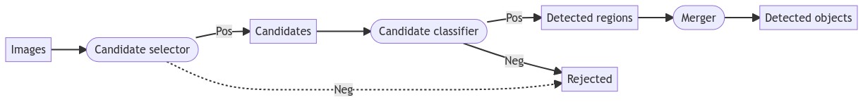
For the first phase, there are two main strategies: either create a very large number of candidates by densely sampling the space of possible bounding boxes, or create a restricted set of candidates, using the image features already in the first phase to reject “obvious” negatives. The main advantage of the first approach is that it generally ensures that no positive object is accidentally rejected in the first phase, and therefore not even presented to the candidate classifier. The main advantage of the second is that it makes the task of the candidate classifier a lot easier.
The overall performance of the whole detection pipeline, however, is not just affected by the performance of the selector, classifier and merger, but also, as in all machine learning tasks, by the selection of the possible data used for the evaluation. In the MITOS12 dataset, the 35 image patches correspond to small portions of 5 WSI, selected because of the presence of several mitosis. When the choice of regions of interest is not random, the distribution of positive & negatives changes with the size of the selected region. Taking a larger region “around” the mitosis that first attracted the attention of the pathologist is likely to increase the proportion of negatives, while taking a narrower region would increase the proportion of positives. Given the sparsity of the objects of interest, the effect can quickly become large.
To quickly simulate how this may affect the results of a detection pipeline, we define a detector with the following characteristics:
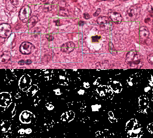
The “candidate selection” step filters out 99.99% of the possible candidates at the pixel level, assuming that we define the set of possible candidates as same-sized patches centred on each pixel of the image (so there are as many possible candidates before selection as there are pixels in the image). This assumes that most possible candidates will be trivially dismissed, which is not unrealistic in a mitosis detection problem, as all pixels that are relatively lighter are certain not to be part of a mitosis (see Figure 4.11).
The “candidate classifier” step has a 99% specificity and 75% sensitivity rate.
We then look at three scenarios. In the first one, we take the characteristics of the MITOS12 dataset (226 mitosis occupying 0.09% of the total pixel area). In the second, we imagine a more restricted set where a smaller region of interest was considered. We look at what happens if, when restricting the total area by half, we keep about 75% of the mitosis. In the third scenario, we do the opposite and double the total area, and simulate that this includes 150% of the original amount of mitosis. The results presented in Table 4.7 show that, while the recall in all cases remains the same (as it is equal to the sensitivity that we fixed as a parameter of the pipeline), the precision varies as the foreground-background imbalance changes. As proportionally more negative examples are shown, the number of false positives can only increase and the number of true positives can only decrease, so the precision and F1-score can only get worse.
| Scenario | Precision | Recall | F1 |
|---|---|---|---|
| MITOS12 distribution | |||
| Smaller region | |||
| Larger region | |||
| MITOS-ATYPIA-14 distribution |
Of course, as long as methods are compared on exactly the same test set, a ranking of the methods based on the F1-Score should still be representative of their relative performance. However, the characteristics of the dataset are still important to keep in mind when interpreting the results, particularly when the same task is measured on different datasets. The MITOS-ATYPIA-14 dataset, for instance, has a much lower ratio of mitosis to total area, with mitosis representing 0.02% of the total area of the patches. A detection pipeline with the same behaviour as the one we simulated on MITOS12 would see its precision fall from 0.55 to 0.18, and its F1-score from 0.63 to 0.29 just by this change of distribution.
It is tempting to see that as the main explanation for the difference in results observed between the two challenges, as the top result for MITOS12 was a 0.78 F1-score, while it was 0.36 for MITOS-ATYPIA-14. There were, however, less participants in the mitosis detection part of the challenge in the 2014 version, and the MITOS12 challenge was also designed with a problematic train/test split, with patches extracted from the same WSI appearing in both parts of the dataset. The difference in the mitosis density is very likely, however, to be a contributing factor.
4.4.2 Imbalanced datasets in classification tasks
4.4.2.1 Extension to other metrics
As noted in section 4.3.3, the analysis of Luque et al. [32] on the effects of imbalanced datasets in classification tasks uses a “detection” F1-Score, which is not a global metric for a classification problem. We therefore reproduce the experiment with the two version of the macro-averaged F1-score, the and the . We also add the , normalized similarly as the (cf. section 4.3.3), for completeness’ sake. Our results are presented in Table 4.8, and a comparison between the biases of the , the , the and the is shown in Figure 4.12.
| Metric | Range of bias |
|---|---|
| [-0.43, 0.16] | |
| [-0.28, 0.14] | |
| [-0.41, 0.49] |
As we can see, the shape of the bias is very similar between the and the . While the is clearly extremely biased with imbalanced datasets and should generally be avoided as a binary classification metric, the use of a macro-averaged version of the metric reduces its bias quite significantly and puts it in the same range as the (see Table 4.6) for the , and even lower for the . The latter therefore appears to be more robust to class imbalance than the MCC.
4.4.2.2 Extension to multi-class problems
In a multi-class problem, the notion of a “positive” and “negative” class has to be removed. The generic parametrized confusion matrix is therefore, for classes:
Where is the total number of samples, is the proportion of class in the dataset, and is the proportion of class samples that were misclassified as class , so that and .
This leads to a parametric space with a very high dimensionality, that is quite complex to explore. For a 3-class problem, we would have two “balance” parameters and (which set ) and six “error distribution” parameters (which set , etc.). In general, for a class problem, we would have balance parameters and error distribution parameters.
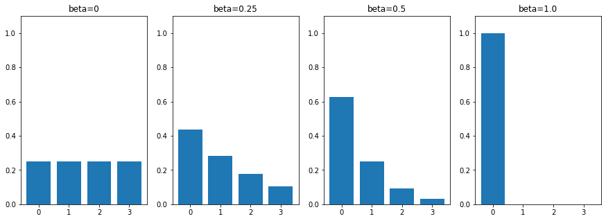
To reduce this dimensionality, we define a single balance parameter that will vary from 0 (balanced) to 1 (extremely imbalanced). We also define , and then recursively and . An example of the class distributions yielded by this method for a 4-class problem and different values is shown in Figure 4.13.
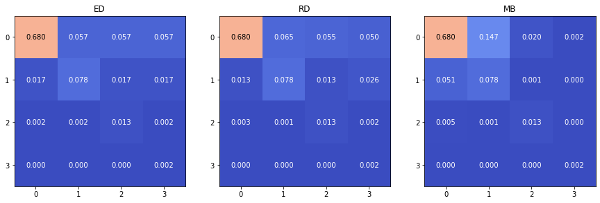
For the error distribution, we consider three scenarios that allow us to only have as parameters the class sensitivity values:
The evenly distributed error (ED) scenario, where we set .
The randomly distributed error (RD) scenario, where we first generate a random “error likelihood” matrix so that and , and the are then simply computed as . The error matrix needs to be computed first so that the same “error likelihood” is used when exploring the space of values.
The majority bias error (MB) scenario, where the errors are distributed more towards the majority class, so that .
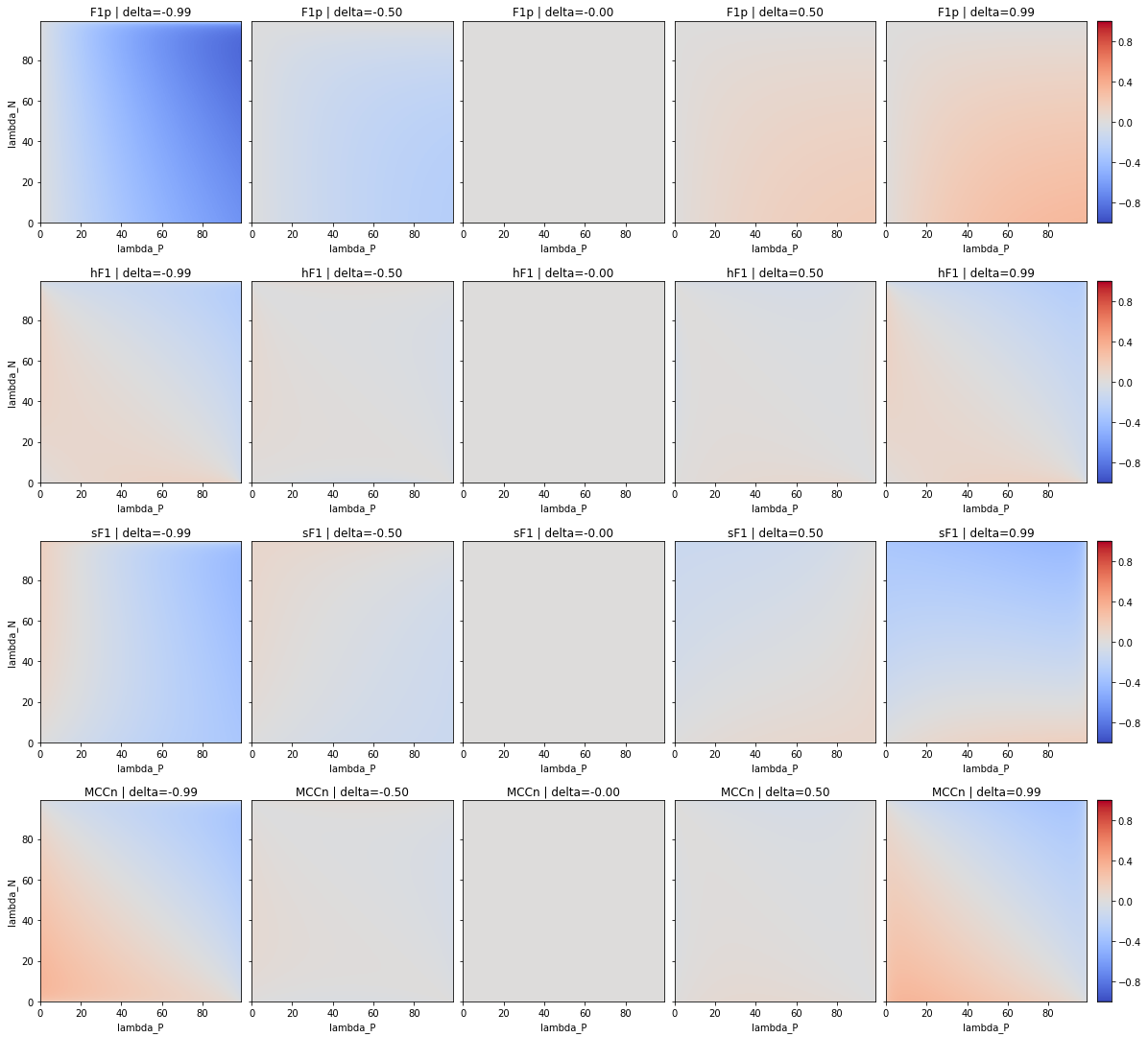
The three scenarios are illustrated in Figure 4.14. The biases related to the class imbalance are reported in Table 4.9 for and , in the three error distribution scenarios. The imbalance bias for the and the increases as the number of classes increases. For the , the main effect seems to be that the negative bias (i.e. the imbalanced result is worse than the balanced result at the same sensitivity values) becomes more important than the positive bias, so the in general will be lower in a multi-class, imbalanced dataset. The keeps a relatively constant bias. The sees the range of its bias reduced, but only on the positive side. Finally, the GM remains unbiased.
| - | [-0.49, 0.49] | [0, 0] | [-0.34, 0.34] | [-0.28, 0.14] | [-0.43, 0.16] | [-0.41, 0.49] |
| ED | [-0.65, 0.65] | [0, 0] | [-0.36, 0.2] | [-0.42, 0.13] | [-0.42, 0.18] | [-0.42, 0.24] |
| RD | [-0.65, 0.65] | [0, 0] | [-0.37, 0.21] | [-0.43, 0.12] | [-0.42, 0.17] | [-0.42, 0.24] |
| MB | [-0.65, 0.65] | [0, 0] | [-0.37, 0.17] | [-0.42, 0.14] | [-0.44, 0.18] | [-0.42, 0.24] |
| ED | [-0.73, 0.73] | [0, 0] | [-0.38, 0.19] | [-0.52, 0.11] | [-0.41, 0.19] | [-0.43, 0.20] |
| RD | [-0.73, 0.73] | [0, 0] | [-0.38, 0.18] | [-0.52, 0.11] | [-0.41, 0.23] | [-0.43, 0.20] |
| MB | [-0.73, 0.73] | [0, 0] | [-0.45, 0.19] | [-0.52, 0.14] | [-0.45, 0.18] | [-0.43, 0.20] |
4.4.2.3 Normalized confusion matrix to counter class imbalance
To counteract the bias induced by class imbalance, the most obvious solution is to compute the metrics on the balanced (or normalized) confusion matrix (NCM). The NCM is computed by simply dividing each element by the sum of the values on the same row:
This acts as a “resampling” of the data so that each class has the same number of samples, while keeping the per-class sensitivity values intact. This solution, however, is not without its own drawbacks. To illustrate these, we need to use some real data. The results of the MoNuSAC 2020 challenge can be used in this case: as the prediction maps of four teams are available, it is possible to compute alternate metrics to those reported in the challenge results.
The MoNuSAC challenge is a nuclei instance segmentation and classification challenge. We will focus here on the classification part of the challenge, which has four classes (epithelial, neutrophil, lymphocyte and macrophage). From the published prediction maps, we can compute the classification confusion matrices (based on the matching pairs of detected nuclei, which will therefore vary between the teams), shown in Table 4.10, and the number of per-class TP, FP and FN for the detection task, shown in Table 4.11. A full description of the MoNuSAC dataset is given in Annex A.
| Team 1 | E | L | N | M | Team 2 | E | L | N | M |
|---|---|---|---|---|---|---|---|---|---|
| E | 6098 | 260 | 8 | 12 | E | 6240 | 88 | 0 | 57 |
| L | 79 | 7214 | 2 | 1 | L | 162 | 7131 | 4 | 6 |
| 6 | 5 | 39 | 118 | 2 | N | 1 | 18 | 133 | 10 |
| M | 16 | 11 | 8 | 170 | M | 16 | 1 | 11 | 164 |
| Team 3 | E | L | N | M | Team 4 | E | L | N | M |
| E | 5960 | 96 | 0 | 1 | E | 6193 | 302 | 2 | 22 |
| L | 76 | 6864 | 3 | 0 | L | 179 | 7274 | 1 | 0 |
| N | 1 | 20 | 137 | 3 | N | 3 | 38 | 117 | 2 |
| M | 30 | 8 | 11 | 159 | M | 30 | 7 | 25 | 155 |
| FP detections | E | L | N | M |
|---|---|---|---|---|
| Team 1 | 1338 | 829 | 14 | 59 |
| Team 2 | 962 | 629 | 5 | 285 |
| Team 3 | 2932 | 1545 | 50 | 99 |
| Team 4 | 1035 | 770 | 10 | 13 |
| FN detections | E | L | N | M |
| Team 1 | 831 | 507 | 8 | 102 |
| Team 2 | 824 | 500 | 10 | 115 |
| Team 3 | 1152 | 860 | 11 | 99 |
| Team 4 | 690 | 349 | 12 | 90 |
| TP detections | E | L | N | M |
| Team 1 | 6378 | 7296 | 164 | 205 |
| Team 2 | 6385 | 7303 | 162 | 192 |
| Team 3 | 6057 | 6942 | 161 | 208 |
| Team 4 | 6519 | 7454 | 160 | 217 |
From these results, we can look at the relationship between the values and the class imbalance. From Table 4.12, we can see that the two majority classes are associated to much higher sensitivity values than the two minority classes. If we are trying to judge how the algorithm would perform “in a world where the data is balanced,” this normalization may therefore not be completely accurate.
| Range | Epithelial | Lymphocyte | Neutrophil | Macrophage |
|---|---|---|---|---|
| Annotations | 0.47 | 0.50 | 0.01 | 0.02 |
| Predicted | [0.46 - 0.50] | [0.47 - 0.52] | [0.01 - 0.01] | [0.01 - 0.03] |
| Detection | [0.84 - 0.90] | [0.89 - 0.96] | [0.93 - 0.95] | [0.63 - 0.71] |
| Classif. | [0.95 - 0.98] | [0.98 - 0.99] | [0.72 - 0.85] | [0.71 - 0.85] |
Another possible problem that may arise from the normalization is that, if we have a very large imbalance with some very rare classes, we may artificially increase what is simply “sampling noise.” To illustrate this, we again turn to the MoNuSAC results. In this experiment, we keep all the properties of the dataset (class distribution of the ground truth) and of each team’s results (detection recall and per-class distribution of classification errors, represented by the ). We then randomly sample N nuclei from an “infinite” pool of samples that has the same class proportions as the ground truth and compute each team’s confusion matrix based on that sampling. On average, we will obtain confusion matrices that are the same as those of the challenge, but we will also be able to see the variation due to random sampling.
In Table 4.13, we report the results from 5.000 runs of the simulation based on 1.000, 5.000 or 15.000 samples (15.000 being close to the real number of annotated nuclei in the MoNuSAC test set). We show, for each classification metric, the maximum divergence observed across the four teams (, with the x percentile) as an uncertainty measure. As we can see, if we have many annotated samples like in MoNuSAC, the uncertainty due to the random sampling remains very low even in the NCM. If we have a smaller set of samples, however, this uncertainty can quickly grow, at least for the and . As the metric is unbiased relative to the imbalance, the results do not change between CM and NCM, but the random sampling uncertainty is very high. The also has a high uncertainty overall.
| 15.000 samples | ||||||
|---|---|---|---|---|---|---|
| CM | 0.001 | 0.003 | 0.001 | 0.006 | 0.001 | 0.001 |
| NCM | 0.003 | 0.003 | 0.002 | 0.003 | 0.002 | 0.002 |
| 5.000 samples | ||||||
| CM | 0.002 | 0.011 | 0.002 | 0.011 | 0.001 | 0.002 |
| NCM | 0.010 | 0.011 | 0.006 | 0.009 | 0.007 | 0.006 |
| 1.000 samples | ||||||
| CM | 0.006 | 0.056 | 0.005 | 0.046 | 0.003 | 0.005 |
| NCM | 0.052 | 0.056 | 0.035 | 0.054 | 0.035 | 0.034 |
Overall, the uncertainty added by using the NCM instead of the CM remains relatively low but, if the sample size is small, it is still in a range that could potentially affect the comparison between algorithms (as many biomedical datasets have much fewer than 1.000 samples available).
4.4.2.4 Conclusions on imbalanced datasets in classification tasks
Given the above analysis, the flowchart presented in Figure 4.15 attempts to summarize how to decide which classification metrics to use based on the class imbalance of the dataset.
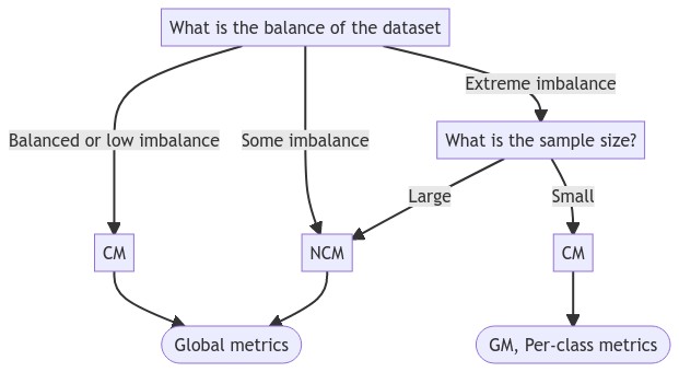
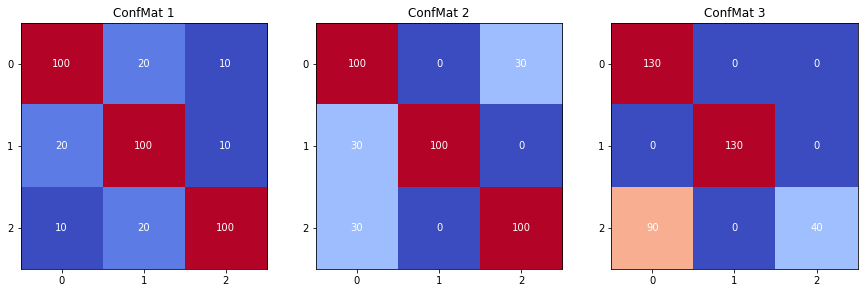
With mostly balanced datasets, the confusion matrix can be used directly to compute any global metrics. Which of these to use will mostly depend on whether the distribution of the errors among the classes is important for the evaluation or not. Figure 4.16 shows three confusion matrices corresponding to a balanced dataset with the same total error, but with different distributions per class. Table 4.14 shows the results of the different global metrics for these confusion matrices.
| \ | ||||||
|---|---|---|---|---|---|---|
| ConfMat 1 | 0.769 | 0.769 | 0.654 | 0.654 | 0.771 | 0.755 |
| ConfMat 2 | 0.769 | 0.769 | 0.654 | 0.660 | 0.783 | 0.780 |
| ConfMat 3 | 0.769 | 0.675 | 0.654 | 0.713 | 0.814 | 0.871 |
Obviously, the accuracy is the same for all three: it is completely independent from how the error is distributed, as long as the total error remains the same. Less obvious is the invariance of the unweighted kappa, which is expected to depend also on the distribution of the predicted classes, which here varies between the confusion matrices. With a perfectly balanced dataset, however, we can show that the is actually independent from the error distribution.
Using the original definition of the kappa:
It is clear that , which is the accuracy, will not vary. Meanwhile, we have for classes and samples:
And, in a balanced dataset:
That is, the sum of each row will be the same. Therefore:
And finally:
Which is illustrated in Table 4.14 with . If there is any class imbalance, this relationship no longer holds true.
The Geometric Mean is equal for the first two confusion matrices, for which the are equal whereas the errors in each class are distributed differently. The Matthews Correlation Coefficient and the two macro-averaged F1 scores, on the other hand, have different values for the three confusion matrices, and are therefore affected by changes in the distribution of errors. Whether this is a desired trait for the metric depends on the task and the evaluation criteria. It is interesting to note, however, that the latter three increase as the error gets progressively more concentrated in the three confusion matrices, even in the third one where all the prediction errors concern one class only. This contrasts greatly with the GM, which penalises the third confusion matrix a lot more, as the much smaller for class 2 will greatly affect the score.
If the dataset is imbalanced but with still a reasonable number of samples of each class (what is a reasonable amount will depend on how much sampling uncertainty is acceptable for the purpose of the evaluation of the task), using the normalized confusion matrix to reduce the problem to a balanced problem is a good solution, with the same choice of metrics available.
In cases of extreme imbalance with a small sample size, where there are very few samples available for the minority class, the normalization may induce too much sampling uncertainty. It is therefore probably advisable in those cases to focus on an unbiased global metric like the GM, or on class-specific metrics separately.
4.4.3 Limit between detection and classification
An interesting aspect of object detection tasks is their close relationship to binary classification tasks. The main difference, in the definition we have used for the task, is that an “object detection” task does not have a countable number of true negatives, but as we have seen a detection pipeline is often composed of a “candidate selection” step and a “classification” step.
The danger of this confusion between detection and classification is that it is tempting to use the confusion matrix of the classification part and its associated metrics to measure the detection performance of an algorithm. For instance, Giusti et al. [17] compare humans and algorithms on a mitosis detection task using pre-sampled image patches forming a balanced dataset, and score them with a ROC curve, which takes the TN into account. To illustrate the impact that the definition of the task has on the evaluation, we simulate four scenarios on synthetic data.
In each scenario, we define five categories of “candidates”:
Negative, trivial (): corresponds to negative candidates from a sampling method that will always be correctly rejected by the classifier.
Negative, easy (: negative candidates that the classifier will rarely fail to reject.
Negative, hard (): negative candidates that are similar enough to the objects of interest that the classifier will regularly misclassify them as positive.
Positive, hard (): positive candidates that are hard to separate from the non-objects and that the classifier will regularly reject.
Positive, easy (): positive candidates that the classifier will rarely miss.
Two of the scenarios correspond to “handpicked” candidates, where in one case negative examples are chosen for being “difficult” to classify, and in the other they are chosen to be easier. We also simulate two “candidate selectors” (see Figure 4.10), the first one a non-specific selector that largely sample the set of possible candidates, leading to many candidates that are trivially easy to reject to be added to the set, while the other simulates a more targeted selector which tends to add more “hard” negative examples but also includes some trivial examples.
Each scenario differs by the number of candidates presented from each category. In all four, the number of and are the same (as they correspond to the positive objects, which will be the same regardless of the “candidate selection” procedure) and is set to 500. In the “Handpicked Hard” scenario, negative examples are added with a majority of and no . In the “Handpicked Easy” scenario, negative examples are added with a majority of and no . Finally, in the “Large selector” scenario, 5000 trivial candidates are added, and . All the values are reported in Table 4.15.
| Scenario | |||||
|---|---|---|---|---|---|
| Handpicked Hard | 0 | 200 | 800 | 500 | 500 |
| Handpicked Easy | 0 | 800 | 200 | 500 | 500 |
| Large selector | 5000 | 800 | 800 | 500 | 500 |
| Targeted selector | 50 | 600 | 800 | 500 | 500 |
We define a single classifier which outputs a random “confidence” value for each class, sampled from a normal distribution with the following characteristics:
The REC, PRE and AP are used as detection metrics, and the SPE and MCC as classification metrics. The results obtained by the “classifier” based on these parameters and using a confidence threshold are reported in Table 4.16.
| Scenario | REC | PRE | AP | SPE | MCC |
|---|---|---|---|---|---|
| Handpicked hard | 0.85 | 0.77 | 0.92 | 0.75 | 0.60 |
| Handpicked easy | 0.85 | 0.93 | 0.98 | 0.94 | 0.79 |
| Large selector | 0.85 | 0.77 | 0.92 | 0.96 | 0.78 |
| Targeted selector | 0.85 | 0.77 | 0.92 | 0.83 | 0.67 |
The REC, which only depends on the positive examples, are equal in all cases. The PRE and SPE, however, are unsurprisingly much larger when the handpicked negative examples are easier. Looking at detection metrics (PRE and AP), the “large selector,” “targeted selector” and “handpicked hard” scenarios are identical. The classification metrics, however, vary widely depending on the scenario, and on which negative candidates were added to the dataset.
This illustrates some of the pitfalls of confusing detection and classification tasks: it may lead to using metrics which are not adapted to the problem. If a manual selection of the candidates is done, it includes a potential bias to the results, as the candidate distribution may no longer be representative of the actual data present in the images in a real situation.
4.4.4 Use of detection metrics for instance classification
As previously noted, the results of an instance classification task can be described with a confusion matrix which combines the detection and classification aspects of the results, with a negative (“no object/background”) class alongside the target classes.
Such problems are often treated as “multi-class detection,” so that detection metrics are computed per target class and then averaged, with for instance a macro-averaged F1-Score ( or ). It should be noted, however, that a “macro-averaged F1-Score” in a multi-class detection problem is not exactly the same as a “macro-averaged F1-score” in a classification problem. In the latter, as there is no “background class,” all the elements on the diagonal are both true positives (of their own class) and true negatives (of the other classes), while all the elements off the diagonal are both false positives (of their “predicted” class) and false negatives (of their “ground truth” class). In multi-class detection, however, this is not true for the elements on the first row (which are each “false positives” of their predicted class only) and for the elements on the first column (which are each “false negatives” of their ground truth class only).
Indeed, this leads to certain biases to these averaged metrics, as they will penalize “misclassifications” more harshly than “missed detections” and “false detections.” To illustrate that, we can start from a “perfect” 2-classes detection confusion matrix with 10 objects in each class:
If we transform one of the correct predictions from class 1 into a “misclassification,” we get:
For the two target classes, the computed TP, FP and FN are:
And therefore:
If the misclassification is transformed into a “missed detection,” we get:
Leading to:
And:
Finally, if, instead of a “missed detection,” we add a “false detection,” we get:
We have two different biases in action here. Falsely positive detections (with no corresponding ground truth objects) are penalized less than falsely negative detections (missed objects). The worse type of error, however, is misclassification. This can lead to very counterintuitive results, as methods that completely miss objects may be ranked higher than methods that find the objects but fail to classify them properly.
To avoid this issue, a better strategy if possible is to separate the two problems into a “single-class” detection problem, where all the “target” classes are grouped into one, and a “multi-class” classification problem, where only the objects that were properly detected are considered. In our example, we therefore obtain detection () and classification () matrices as follows:
And:
The detection and classification metrics can then be computed separately. The advantage of this approach is that it makes it immediately clear what the specific weaknesses of the algorithm are. The “missed detection” and “false detection” cases will both have an imperfect detection score, but a perfect classification score, while the “misclassification” case will have a perfect detection score but an imperfect classification score. The insights that we gain from the evaluation metrics are therefore much improved, and the ranking of the methods can be adjusted according to the needs of the clinical application being considered. This is particularly appropriate if the target classes are naturally part of a “superclass”: for instance, the “epithelial,” “lymphocyte,” “neutrophil” and “macrophage” classes of MoNuSAC can be grouped into a “nuclei” superclass for the purpose of measuring the detection performance.
4.4.5 Agreement between classification metrics
There is a large diversity of classification metrics, and it can be difficult to really get a sense of their levels of agreement or disagreement. To quantify inter-metrics agreement, we perform a simple experiment. A synthetic dataset is constructed with some randomized features: the number of classes, the size, the number of features, the difficulty, and the imbalance. A Support Vector Machine (SVM) classifier is trained on 90% of the samples and tested on the remaining 10%. The values of the different classification metrics are then computed on the predicted test set. This experiment is repeated 50 times, leading to 50 values for each metric. The Spearman correlation coefficient between each pair of metrics is then computed to form a “similarity matrix,” which is shown in Figure 4.17. Such a matrix is, however, not particularly easy to interpret. Two interesting ways of visualising the (dis)similarity are Multi-Dimensional Scaling (MDS) [5] and dendrograms.
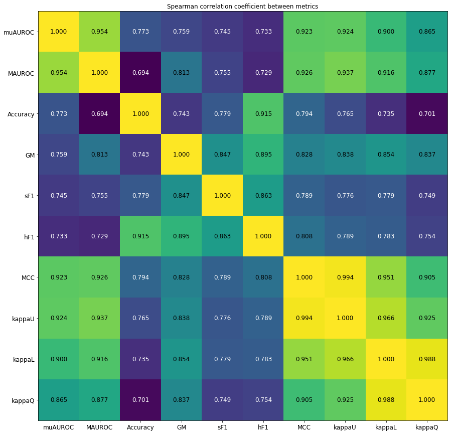
Dendrograms (see Figure 4.18) are very useful to quickly visualize clusters from a dissimilarity matrix and are for instance used to compare classification metrics in a study by Ferri et al. [12], and to visualize the similarity of different tasks based on challenge results by Wiesenfarth et al. [44].
![Figure 4.18. Dendrogram visualisation of the similarity matrix shown in Figure 4.17, using the “average” (UPGMA) inter-cluster dissimilarity update method (as implemented in the Scipy library) [36].](./fig/4-18.png)
With MDS (see Figure 4.19), the dissimilarities (defined here as , with the Spearman correlation coefficient) are projected into a 2D space so that the distance between the points on this 2D space correspond, as much as possible, to the computed dissimilarities. This was proposed by Bouix et al. [6] as a way to evaluate classifiers without a ground truth, but it is an interesting way to visualize (dis)similarities in general.
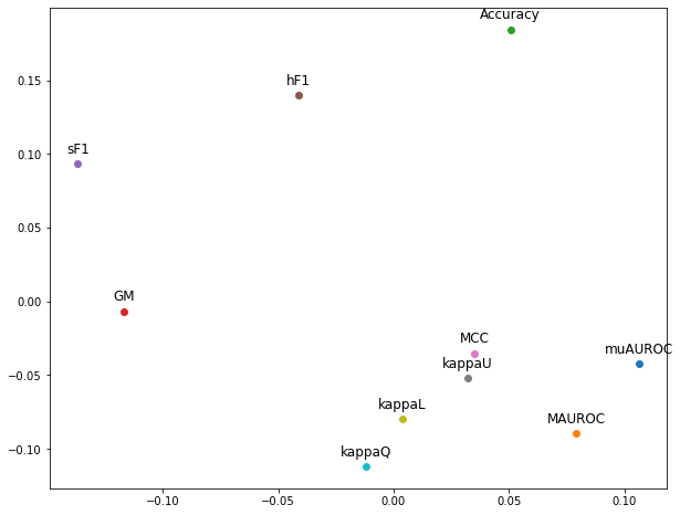
These figures clearly show that the MCC and are the most similar metrics and mostly behave identically, with the often relatively close and the joining them in a loose cluster. The ACC and hF1 also tend to be relatively close to each other, as do the and . The and are further apart from every other metric.
4.4.6 Biases of segmentation metrics
Overlap-based metrics and distance-based metrics behave very differently with regards to the characteristics of the segmented objects, and in particular with their relative size. Overlap-based metrics, for instance, will be invariant to a rescaling of both prediction and ground truth masks. A distance-based metric, meanwhile, will be rescaled as well if it is expressed in pixels. Whenever possible, these metrics should therefore be expressed in distances on the physical sample (for instance, in µm).
4.4.6.1 Effect of small object size on overlap metrics
Overlap-based metrics, however, tend to be very sensitive to small prediction errors when the objects of interest have very small areas. Because of the fuzziness of the object borders in many digital pathology tasks, any predicted segmentation, even accurate, is likely to have some misalignment in the pixels around the border of the object. This will cause a number of FP and FN pixels that will tend to be correlated to the perimeter of the object. The TP region, meanwhile, will tend to be correlated with the object area. As the ratio will generally be higher for smaller objects, the corresponding IoU will therefore tend to be lower, even for a very good segmentation. For objects which are very small even at high levels of magnification, such as nuclei, this can lead to very problematic results. A shift of a single pixel of the annotation contour (which could correspond to a small bias of the annotation stylus, for instance) can have a very large impact on the IoU, as shown in Figure 4.20. On a lymphocyte with an area of around 300px, the single pixel shift brings the perfect IoU of 1.0 down to 0.88, even though it is arguably as “exact” as the original given the fuzzy nature of the actual border, while a 4px shift brings it down to 0.59, close to the typical matching threshold of 0.5. For the much larger (around 10000px) macrophage, the single pixel shift has an almost perfect IoU of 0.98, and the 4px shift only brings it down to 0.91.
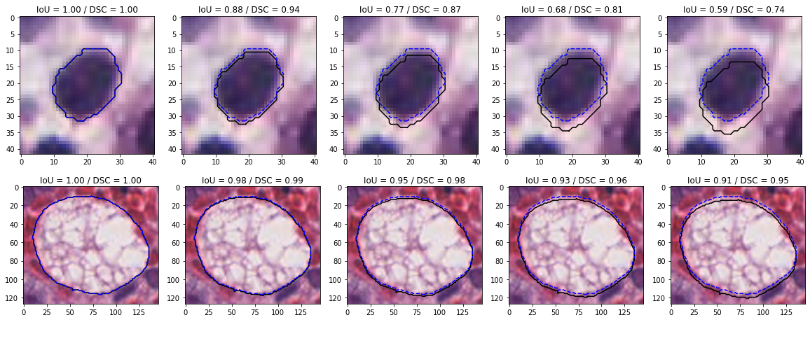
If we look at all the annotated objects in the MoNuSAC dataset, we can plot the relationship between their area and this “single pixel shift” IoU, as shown in Figure 4.21. Once objects are smaller than a ~2.500px area, single pixel shifts start dropping the IoU very quickly. The IoU obtained in the different classes of the dataset therefore has a very different interpretation, as an IoU of 0.8 for a (large) macrophage would correspond to a much “worse” segmentation than for a (small) lymphocyte.
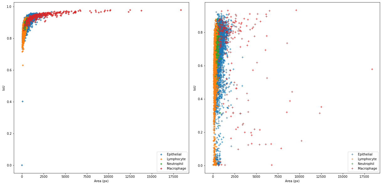
A possible solution to this problem is to include the uncertainty into the computation of the metrics. Similarly to the and defined in section 4.1.4, we can define uncertainty-aware version of the IoU and DSC. If we define the “outer object” and the “inner object” , we can redefine the per pixel TP, FP and FN as:
And therefore:
The results of this uncertainty-aware overlap metrics are illustrated in Figure 4.22 for , showing that the and remain high when the prediction stays within the uncertainty region.
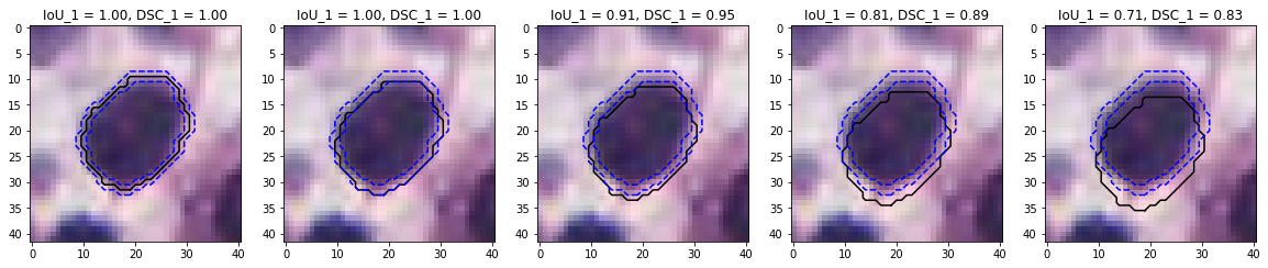
To explore how the characteristics of the IoU on small objects can affect the performance evaluation of competing algorithms, we turn to the MoNuSAC challenge results. The evaluation metric used in MoNuSAC is the Panoptic Quality, which includes the IoU as a “segmentation” component. Several examples of the results from the four teams whose predictions are available on nuclei of different types are shown in Figure 4.23. On the first row, Team 3 and 4 are harshly penalized for having very slightly overestimated the size of the object compared to the ground truth. Team 3’s segmentation only gets an IoU of 0.57, while Team 4, which is still very good, is near the 0.5 matching threshold used in the challenge. On the other hand, Team 1 and 2 are not penalized by their more biologically problematic shape mismatch.
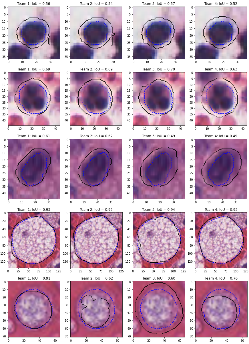
In the second row, the four predictions are mostly equivalent, yet there is still a wide range of IoU, from 0.63 to 0.70 for Team 3, which provides the least similar overall shape and yet the best score. On the third row, Team 3 and 4 both fall under the 0.5 matching threshold, largely due to the fact that the annotation appears to be slightly off to the right and bottom. On the fourth row, we see that for a much larger object the score are a lot higher, despite a segmentation that is not necessarily “better” biologically than those of the smaller objects above. On the last row, we see that for those larger objects the differences between the teams’ results make a lot more sense, but still fail to recognize the more meaningful types of errors, such as the bad shape of Team 2’s result, compared to the size overestimation by Team 3. The HDs computed on the last rows yield results of 3.0, 13.6, 9.0 and 9.2px respectively, more accurately capturing in this case the problematic nature of Team 2’s results.
If we look at the IoUs per cell class in Figure 4.24 for one of the participating teams, it is clear that while the segmentation score for the lymphocytes is lower than for the other classes, using the uncertainty-aware version of the score makes the results even across the classes. This indicates that the poor results for the lymphocytes may be largely due to the fuzziness of the annotations combined with the small size of the objects, rather than to the quality of the predicted segmentation.
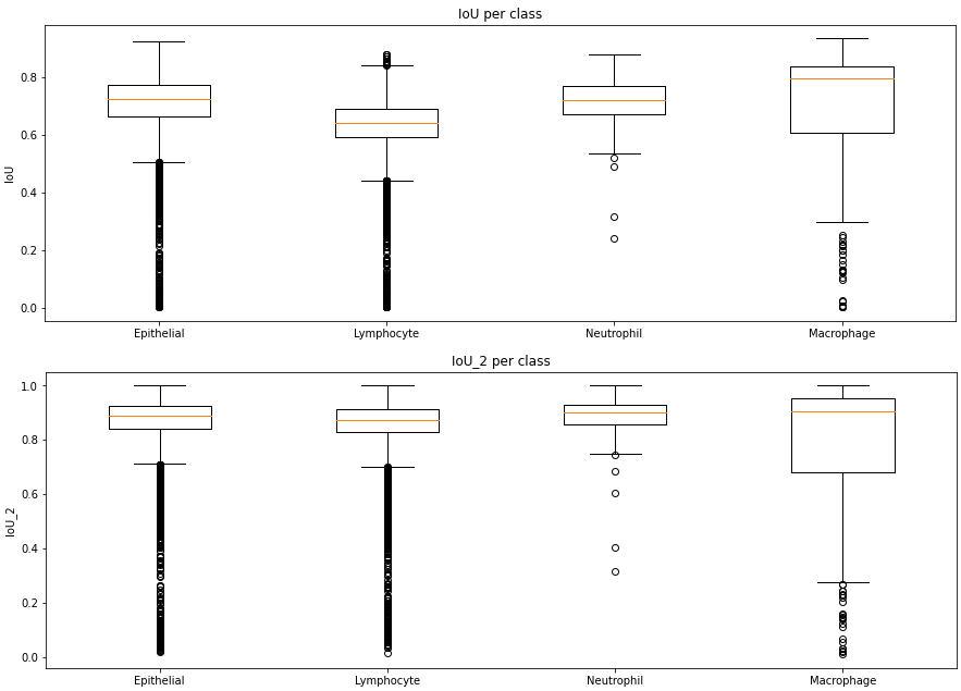
4.4.6.2 Over- and under-estimation of objects sizes
Overlap metrics have another bias that should be noted: they do not penalize in the same way over- and under-estimation of the sizes of the objects. This can be easily shown using the formulation of the metrics based on the TP, FP and FN. If, starting from a perfect prediction () we add “background” pixels to the predicted positives (corresponding to an overestimation of the object size), we have , and:
Whereas if we remove the same number of pixels from the true positives, we have , and:
Therefore, for an equal number of erroneous pixels, we have a bias equal to:
This means that there is a bias in favour of “overestimation” of the object size, which is proportional to the size of the error and inversely proportional to the true size of the object. This effect is clearly visible in Figure 4.25. In the top plot, we can see that for a fixed error of 20px, the bias in favour of overestimation becomes clear as the object area gets smaller. In the bottom plot, we can see that the bias increases as the size of the error increases for a fixed object area.
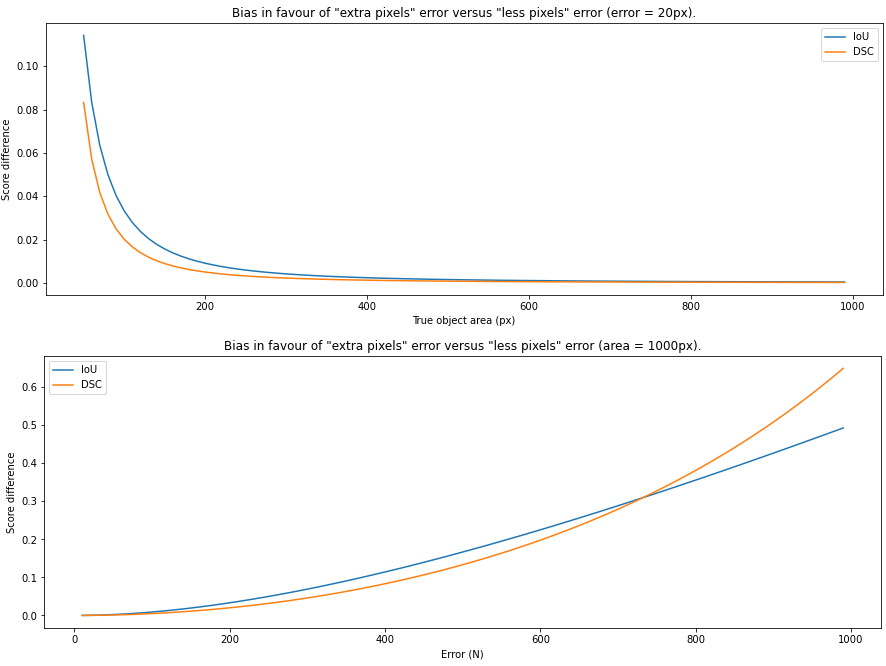
4.4.7 Multi-metrics aggregation: study of the GlaS 2015 results
To aggregate individual metrics into a single final ranking, one solution is to first rank the metrics separately, then to combine them using, for instance, the “sum of ranks.” This approach was notably used by the GlaS 2015 challenge for gland segmentation. The main advantage is that the separate ranks provide a more insightful interpretation of the results when comparing different algorithms. It also makes it possible to combine rankings that have a completely different scale, such as the DSC and the HD. An important weakness, however, is that the “final score” of an algorithm (which is the sum of ranks) becomes dependant also on the results of the other algorithms being compared, and overall rankings may be undesirably affected by which methods are included in the study. It also does not differentiate between a case where most methods are essentially equivalent according to a metric to a case where some methods are largely better or worse. This is apparent in the table of results from the GlaS 2015 challenge, which we reproduce in Table 4.17. Six separate rankings are computed, on three metrics and two separate test sets. Some of the difference in ranks, however, come from very small differences in metrics which are very unlikely to be significantly different and, for the segmentation metrics, are probably well within the uncertainty on the border position. For instance, for the HD in Part A, ranks 3-6 are within a single pixel distance, and in DSC part B ranks 2-5 are within the same percent. A very slight difference in the annotations could easily change the rankings of #2 and put it in first place or in third.
| Team | Rank sum | ||||||
|---|---|---|---|---|---|---|---|
| - | Part A | Part B | Part A | Part B | Part A | Part B | |
| #1 | 0.912 (1) | 0.716 (3) | 0.897 (1) | 0.781 (5) | 45.42 (1) | 160.3 (6) | 17 |
| #2 | 0.891 (4) | 0.703 (4) | 0.882 (4) | 0.786 (2) | 57.41 (6) | 145.6 (1) | 21 |
| #3 | 0.896 (2) | 0.719 (2) | 0.886 (2) | 0.765 (6) | 57.35 (5) | 159.9 (5) | 22 |
| #4 | 0.870 (5) | 0.695 (5) | 0.876 (5) | 0.786 (3) | 57.09 (3) | 148.5 (3) | 24 |
| #5 | 0.868 (6) | 0.769 (1) | 0.867 (7) | 0.800 (1) | 74.60 (7) | 153.6 (4) | 26 |
| #6 | 0.892 (3) | 0.686 (6) | 0.884 (3) | 0.754 (7) | 54.79 (2) | 187.4 (8) | 29 |
| #7 | 0.834 (7) | 0.605 (7) | 0.875 (6) | 0.783 (4) | 57.19 (4) | 146.6 (2) | 30 |
| #8 | 0.652 (9) | 0.541 (8) | 0.64 (10) | 0.654 (8) | 155. (10) | 176.2 (7) | 52 |
| #9 | 0.777 (8) | 0.31 (10) | 0.781 (8) | 0.617 (9) | 112.7 (9) | 190.5 (9) | 53 |
| #10 | 0.64 (10) | 0.527 (9) | 0.737 (9) | 0.61 (10) | 107.5 (8) | 210. (10) | 56 |
A possible solution could be to allow for ex aequo rankings when results are within a certain tolerance of each other. A difficulty, however, is that for instance rank #1 and #2 may be within the ex aequo tolerance, and rank #2 and #3 as well, but not rank #1 and #3. To get around that problem, we can use a statistical score that replaces the “rank” by a score corresponding, for an algorithm A, to the number of other algorithms that are significantly worse (according to an adequate statistical test, as discussed in section 4.3.4) to which we subtract the number of other algorithms that are significantly better. This number can then be summed across the metrics and/or datasets. The resulting statistical score will be higher for algorithms which are often significantly better than their counterparts. This method was introduced in one of our publications [13].
As we do not have the detailed per-image results of the GlaS challenge, we cannot perform these tests, but we can get an idea of what the results can look like using some basic heuristics. Let’s assume that any F1-Scores or DSC value pairs that differ by more than 0.05 are “significantly different,” as are any HD value pairs that differ by more than 5 pixels. Applied to Table 4.17, this would give us the results presented in Table 4.18. This method provides a relatively easy interpretation of the scores: any method that has a negative score is, on average, significantly worse than most other methods. As this is true regardless of the number of methods considered, it is easier to see method which can safely be discarded as underperforming (in this case, #8-#10). Meanwhile, metrics where the results were extremely close no longer contribute much to the overall standing: according to the DSC, for instance, we can see quickly see that methods #1-#7 are essentially equivalent. There is also a big reward for methods that manage to be significantly better than all or most others in one of the rankings, like #1 on HD Part A, #5 on Part B or #2, #4 and #7 in HD Part B.
The overall ranking based on the score sum shows some small changes, with #2 having the best scoring, followed by #1 and #4, and then #3 and #5. This mostly acknowledges that #3 was “lucky” in the rankings of the challenge, as they tended to be at the “front” of groups of mostly identical results, and therefore may have seen their overall ranking artificially improved. This is, however, just an illustration of how the insights on the challenge results may change when using such a scoring method and should not be considered as an “alternative ranking” of the challenge results, as this would require access to the per-image results of the different teams.
| Team | Rank sum | ||||||
|---|---|---|---|---|---|---|---|
| - | Part A | Part B | Part A | Part B | Part A | Part B | |
| #1 | 4 | 3 | 3 | 3 | 9 | 0 | 22 |
| #2 | 4 | 3 | 3 | 3 | 3 | 7 | 23 |
| #3 | 4 | 4 | 3 | 3 | 3 | 0 | 17 |
| #4 | 3 | 3 | 3 | 3 | 3 | 7 | 22 |
| #5 | 3 | 8 | 3 | 3 | -3 | 3 | 17 |
| #6 | 4 | 3 | 3 | 3 | 3 | -6 | 10 |
| #7 | -1 | -3 | 3 | 3 | 3 | 7 | 12 |
| #8 | -8 | -6 | -9 | -7 | -9 | -3 | -42 |
| #9 | -5 | -9 | -6 | -7 | -7 | -6 | -40 |
| #10 | -8 | -6 | -8 | -7 | -5 | -9 | -41 |
4.4.8 Why panoptic quality should be avoided for nuclei instance segmentation and classification
The notion of “Panoptic Segmentation,” and its corresponding evaluation metric “Panoptic Quality” (PQ), was introduced by Kirillov et al [27]. Panoptic segmentation, per Kirillov’s definition, attempts to unify the concepts of semantic segmentation and instance segmentation into a single task, and a single evaluation metric. In Panoptic Segmentation tasks, some classes are considered as stuff (meaning that they are regions of similar semantic value, but with no distinct instance identity, such as “sky” or “grass”), and some as things (countable objects). The concept was initially applied to natural scenes using the Cityscapes, ADE20k and Mapillary Vistas datasets. It was then applied to the digital pathology task of nuclei instance segmentation and classification in the paper that introduced the HoVer-Net deep learning model [20].
The PQ was then adopted as the ranked metric of the MoNuSAC 2020 challenge [43], then the CoNIC 2022 challenge [19], and has been adopted by several recent publications [18], [23]–[30]. It combines a “recognition metric” and a “segmentation metric” into a single score. It uses the IoU both for the matching rule, which only recognizes matches if the IoU is strictly above 0.5, and as the segmentation metric. As we previously showed, this can lead to very problematic results when applied to nuclei segmentation, as the target objects tend to be very small. Besides the IoU problem, however, there are other fundamental issues with the metric which we will discuss here:
- The PQ in used in digital pathology on instance segmentation and classification tasks, but these tasks are fundamentally different from the panoptic segmentation task that the metric was designed to evaluate.
- The summarization of the performances of a complex, multi-faceted task into a single entangled metric leads to poor interpretability of the results.
4.4.8.1 Panoptic segmentation vs instance segmentation and classification
In the original definition of a “Panoptic Segmentation” problem in [27], each pixel of an image can be associated with a ground truth class and to a ground truth instance label . A pixel cannot have more than one class or instance label (i.e. no overlapping labels are allowed), but a pixel does not necessarily have an instance label (i.e. can be undefined). The distinction between things and stuff therefore becomes that stuff are the classes that do not require instance labels, while things are classes that do require them.
In the HoVer-Net publication [20], the PQ is used for nuclei instance segmentation only, with all “nuclei” classes grouped into a superclass, and a separate “instance classification” metric which similarly combines detection and classification accuracy (as ) where is the detection F1-Score on the nuclei superclass and is the classification accuracy computed on all correctly detected instances. In subsequent uses of the PQ from the same group [18], [19] and in the MoNuSAC challenge, however, the multi-class PQ is used for the whole instance segmentation and classification task.
The first problem of the PQ in digital pathology is that nuclei instance segmentation and classification, is not a panoptic segmentation task. Panoptic segmentation is characterized by two key factors:
- Every pixel is associated with one single class label.
- Every pixel is associated with one single optional instance label.
In instance segmentation and classification, however, the class label is also optional, as there is typically a “background class” that corresponds to everything that is not an object of interest (which can be the glass slide itself, or simply tissue areas that are not part of the target classes). Additionally, if a pixel is associated with a class label, it also needs to have an instance label (i.e. there is no stuff, only things, using Kirillov et al’s terminology), as illustrated in Figure 4.26.
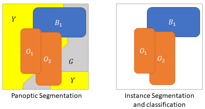
This by itself is not necessarily a problem. Metrics can find uses outside of their original, intended scope: the IoU is generally traced to Paul Jaccard’s study of the distribution of flora in the Alps [24], long before “image segmentation” was on anyone’s radar. There is, however, a problem with the transition between tasks in the present case. The “Recognition Quality” in Kirillov et al’s definition corresponds to the classification F1-Score, whereas the “Detection Quality” in Graham et al’s definition [20] is the detection F1-Score. As we discussed before, there is a key difference between the confusion matrices associated with detection and classification problems, with the presence or absence of the background class. The application of the F1-Score to a classification problem leads to the bias that a higher penalty is given to a good detection with the wrong class (which will be counted as a “false negative” in the ground truth class, and as a “false positive” in the predicted class) than to a missed detection (which will only be a “false negative” in the ground truth class), as previously demonstrated in section 4.4.4, and this bias is therefore transmitted to the PQ.
Figure 4.27 illustrates this problem. In this example from the MoNuSAC results, Team 3 is the only one to detect the nucleus of a macrophage. However, they misclassify it as an epithelial cell. Team 3’s detection is therefore counted both as a false positive for the epithelial class, and as a false negative for the macrophage class. In contrast, the three other teams that did not detect it are only penalized for the macrophage false negative. In a real panoptic segmentation problem, this could not happen, as there is no “background” class: any false negative is always a false positive of another class, as there must be some predicted object or region at that particular location.
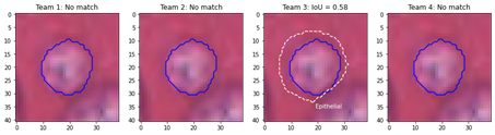
4.4.8.2 Intersection over Union for digital pathology objects
The reliance of the PQ on the IoU impacts it at two levels: the matching rule and the segmentation quality. For the matching rule, it means that the conjunction of a small object and an algorithm that underestimate its size can easily lead to “false false detections,” where clearly matching objects are rejected due to an IoU under 0.5. For the segmentation quality, the problem lies with the interpretability, and with the aggregation. When objects of different classes have different sizes, the limit of what would constitute a “good” IoU within that class are different. When the PQ are averaged between the classes, this therefore adds a hidden “weight” to the metric. Indeed, algorithms that perform poorly on classes with smaller objects will necessarily tend to have a lower average IoU (and therefore PQ) than those that perform poorly on classes with larger objects.
Additionally, it is well known that the IoU does not consider the shape of the object (like other overlap-based metrics such as the DSC). As demonstrated in [40] and shown in Figure 4.23, predictions that completely miss the shape of the object can end up with the same IoU as predictions that match the shape well, but are slightly offset, or slightly under- or overestimate its size. To get a better sense of the segmentation performance of an algorithm, it is often useful to refer both to an overlap-based metric like the IoU and to a border distance metric such as Hausdorff’s Distance (HD). By using the PQ, an important aspect of the evaluation is therefore completely missed. In digital pathology tasks, the shape of the object of interest is often very relevant to the clinical and research applications behind the image analysis task. It is therefore ill-advised to base a choice of algorithm on a metric that ignores that particular aspect.
4.4.8.3 Interpretability of the results
As we have shown in [16], the PQ metric hides a lot of potentially insightful information about the performances of the algorithms by merging together information of a very different nature. While the SQ and RQ have the same range of possible values, being bounded between 0 and 1, the implication of multiplying these values to get the PQ is that the impact of a change in SQ by a factor is exactly the same as a change of RQ by the same factor.
The significance of these changes for the underlying clinical applications, however, can be very different. A 10% reduction in the SQ may only indicate a small underestimation of each segmented object’s size (which, for small objects, would probably be within the typical interobserver variability), whereas a 10% reduction in the DQ indicates potentially much more significant errors, with entire objects being added as false positives, or missed as false negatives. The interpretation of the relative change in SQ is dependent on the size of the ground truth object, while the interpretation of the relative change in RQ is more likely to depend on the class distribution. Ranking different algorithms with the PQ therefore leads to results that cannot really be related to the needs of clinical applications.
4.5 Recommendations for the evaluation digital pathology image analysis tasks
In this chapter, several important aspects of evaluation processes have been highlighted. An attempt will now be made to extract some practical recommendations on how to properly assess the performances of algorithms in a digital pathology context. It should be noted here that, at this stage, we do not yet include in these recommendations the aspects related to interobserver variability, imperfect annotations, and quality control, as those will be considered in the next chapters. Instead, we consider here that we have access to a dataset with annotations that are treated as a mostly correct “ground truth,” outside of a small uncertainty on the boundaries of the objects.
These recommendations follow five axes: the choice of metric(s) depending on the task, the benefits of using simulations to provide context for the results, the importance of using disentangled metrics to independently assess the individual “sub-tasks,” the necessity of proper statistical testing, and the benefits of going beyond the “ranking” paradigm. Other important recommendations for biomedical image analysis challenge organizers can be found in the BIAS guidelines by Maier-Hein et al. [33], and some recommendations for digital pathology evaluation have also been proposed by Javed et al. [25].
4.5.1 Choice of metric(s)
While Figure 4.15 focused on the choice of classification metrics depending on the class imbalance, the expended flowchart in Figure 4.28 attempts to summarize the factors that impact the choice of metric(s) depending on the type of task and the characteristics of the dataset. Such a flowchart is bound to be incomplete, but it highlights some of the main questions that need to be asked when deciding how to evaluate algorithms.
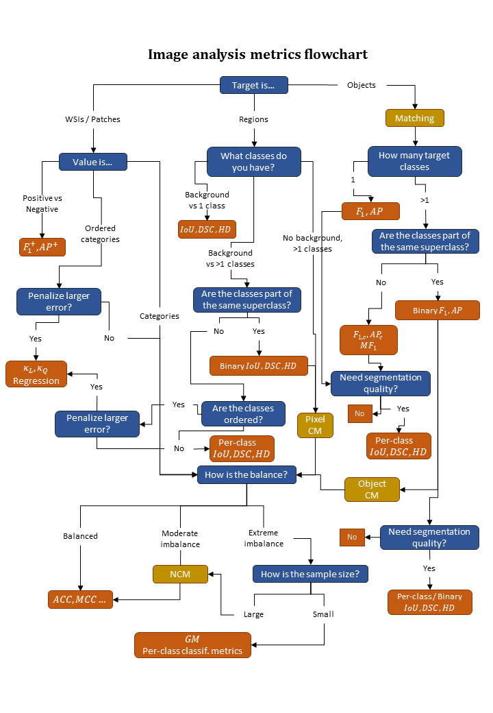
The first of those questions relate to the nature of the target: are there image-level (patch or WSI/patient) labels, regions of interest, or distinct objects to be found? Are there one or more ‘positive’ or ‘target’ class(es) compared to a ‘background,’ ‘others’ or ‘negative’ class, or are all categories considered equal? Are the categories ordered? Is there some “hierarchy” in the classes, so that the target classes can be grouped into one or more “superclass?”
As we move further down the flowchart, questions also relate to what information or insight we are trying to gain from the experiment, as well as the characteristics of the dataset: do we want to penalize larger errors with ordered categories? Do we care about the quality of the segmentation? Is the dataset balanced?
It should be noted that it is possible to end up with several answers when dealing with complex tasks, which illustrates the importance of computing multiple metrics to evaluate all the important aspects of the task. For example, in an instance segmentation and classification problem, following the flowchart from the “objects” target, we could conclude that we need to compute the binary detection or on a “superclass,” then use the object confusion matrix to compute an Accuracy or MCC, and measure the segmentation quality using the per-class IoU, DSC or HD.
The final choice for a specific metric within the same “endpoint” of the flowchart would further depend on the precise characteristics of the dataset and of the real-world application that the dataset attempts to represent. For instance, as we discussed before, very small objects of interest would make the use of overlap-based segmentation metrics inadvisable.
To help in that final choice, and to help contextualize the results, simulations can be used.
To illustrate the use of the flowchart, we can look at the task of nuclei instance segmentation and classification. At the top of the chart, we first ask the nature of the target: in this case, objects (nuclei). The chart thus indicates a first point of attention in the evaluation metric: the matching criterion. The next question then relates to the number of classes, which will be superior to one (as we want to classify different types of cell nuclei), but the classes belong to the same superclass (nuclei). The chart thus recommends using binary detection metrics (such as and ) on the “superclass versus background” detection problem. Two paths can now be further followed. The first one recommends computing the confusion matrix for the classes of the detected objects and then, depending on the (im)balance of the dataset, to compute classification metrics either on the normalized or on the original confusion matrix (or, in extremely imbalanced cases, to stick to per-class metrics such as SPE…). The second path asks if we need to evaluate the segmentation quality, which we do. It therefore recommends the use of per-class and/or binary segmentation metrics. Which one to use will depend on the exact characteristics of a given dataset.
4.5.2 Using simulations to provide context for the results
Most evaluation metrics appear to be easily interpretable at a surface level. Their range is often strictly bounded, and very often presented as a “percentage” (outside of distance-based segmentation metrics). This can give the illusion of metrics providing an absolute scale, with “50%” neatly splitting “failure” from (limited) success, and results above “90%” or “95%” being perceived as very good.
As shown in this chapter, however, evaluation metrics are highly susceptible to differences in the characteristics of the dataset. Even within the same well-defined task, the performance of an algorithm may vary considerably depending on the composition of the test set. Several simulations have been used in this chapter to illustrate some of those differences. Such simulations can be very useful in general to provide context to the results and to help in the choice of metrics and correct interpretation of their values.
Two main types of simulations have been used here: alterations to the annotations, and simulations of performances. In the first type, small changes are done to the annotations to determine how quickly the evaluated performance deteriorates given different types of errors. If done on different metrics, this can help choose which metrics penalize the types of errors that are more relevant to the real-world application under consideration. In the second type of simulation, the performance of a “fake” algorithm is probabilistically pre-determined (with, for instance, distributions of per-class sensitivities), and results are randomly computed based on the known characteristics of the dataset (such as the class imbalance). Multiple simulated runs can provide an indication on the effects of random sampling, and the range of results on the metric being considered that would correspond to that performance level.
4.5.3 Disentangled metrics
It is clear from our experiments and analyses that metrics that attempt to capture multiple aspects of a task in a single score should be avoided. While they may provide an easy way of ranking algorithms, they do so at the cost of interpretability, and produce ranking that cannot reliably be related to the real-world applicability of the results.
If a single ranking for a complex task is desirable, then subtasks should first be ranked independently, and then combined. Ideally, these ranking should take into account the uncertainty of the metric, so that close results can be considered “ex aequo.”
The uncertainty due to the random sampling of test set examples can for instance be captured through adequate statistical tests.
4.5.4 Statistical testing
Deep learning algorithms are full of randomness, from the initialization process to the training itself. Coupled with the randomness inherent in the selection of data samples for the dataset (and in the split between training and test set), this makes it difficult to draw definitive conclusions about small differences in results between algorithms.
Statistical testing provides a way of bringing some objectivity to this interpretation of the difference in results. To compare multiple algorithms based on an arbitrary metric, the Friedman test with a post hoc such as the Nemenyi test are recommended, with the “samples” being either the patients or the image patches (if they are reasonably similar in sizes, to avoid giving too much importance to small errors in small images).
4.5.5 Alternatives to ranking
When evaluating sets of algorithms on a digital pathology task, it is important not to get focused so much on the ranking that we forget the point of the experiment. In most deep learning experiments on digital pathology today, the goal is not yet to validate a product for clinical use, or to find the absolute best trained model to solve a particular task. Rather, the goal is to gather knowledge and insights on the algorithms themselves, to guide future research that may eventually lead us towards methods that bring us closer to clinical applicability.
Rankings can certainly help with providing some insights on the performances of the algorithms, but they are neither sufficient nor necessary in this regard. Alternatives to ranking should are therefore recommended to better capture the behaviour of the methods being compared. Such alternatives include using similarity metrics not just between the methods and the ground truth (particularly when this ground truth, as is often the case in digital pathology, is imperfect and uncertain), but also between the methods themselves. Representations of these similarities can be made using methods such as Multi-Dimensional Scaling or dendrograms, so that the relations between the choices in hyper-parameters and the behaviour of the methods can be better understood.
Clusters of similarly behaved methods can then be found, which can provide additional insights as to which hyper-parameters and which elements of the deep learning pipeline have a larger effect on the performances of an algorithm, as well as what that effect is.
4.6 Conclusion
To conclude this chapter, it is important to note once again that this analysis of the evaluation metrics and processes considered that the ground truth of the task is known and considered as reliable. As we will see in the following chapters, this assumption can be questioned for digital pathology datasets (as for other fields based on medical imaging). To the uncertainties related to random sampling and the inherent biases of the metrics should therefore be added the uncertainties related to the unreliability of the data.
As we move further into the specificities of digital pathology datasets and their effect on the training and evaluation of deep learning algorithms, however, we should always keep in mind the lessons that we have already drawn here.
https://digestpath2019.grand-challenge.org/Dataset/ (Archive link 19/04/2022)↩︎
See classification metrics. It is unclear how the “true negatives” are counted.↩︎
Similar to AP, but with average REC computed for different numbers of FPs.↩︎
AP computed at a minimum IoU threshold of 0.5 for a match.↩︎
Points are given for a sample as , so that correct predictions give one point, predictions that are incorrect by one give zero point, and predictions that are incorrect by two give minus one point, with the ranking based on the sum of points. This is therefore equivalent to an “accuracy” with penalty points for larger errors.↩︎
With a slight modification which does not impact the ranking: ↩︎
are weighted based on the class distribution so that minority classes have less impact on the final score.↩︎
Adapted to include a “detection” aspect, as explained in section 4.1.5.↩︎
Idem↩︎
Unclear, as will be explained in the Quality Control chapter (Chapter 8).↩︎
Which in this case did not specify if it was the linear or quadratic version, which is another problem altogether…↩︎
https://docs.scipy.org/doc/scipy/reference/generated/scipy.cluster.hierarchy.linkage.html↩︎