---- 1.1 The roots of deep learning
------ 1.1.1 Computational model of the neuron
------ 1.1.2 The perceptron and connectionism
------ 1.1.3 Convolutional networks
------ 1.1.4 Backpropagation and stochastic gradient descent
------ 1.1.5 The vanishing gradient and "deep" improvements
------ 1.1.6 The Deep Learning revolution
---- 1.2 Defining deep learning
---- 1.3 Computer vision tasks
---- 1.4 The deep learning pipeline
------ 1.4.1 Data acquisition
------ 1.4.2 Data preparation
------ 1.4.3 Training of a deep learning model
------ 1.4.4 Post-processing
------ 1.4.5 Evaluation
---- 1.5 Deep model architectures
------ 1.5.1 Layers
------ 1.5.2 Macro-architectures: how networks adapt to tasks
------ 1.5.3 Micro-architectures: infinite choices
---- 1.6 Lost in a hyper-parametric world
---- 1.7 Conclusions
1. Deep learning in computer vision
Deep learning has often been described as a revolution: in academic writing [40], [8] in books [67], [32] and in the media.1 The state of the art of computer vision is filled with deep learning algorithms, and this revolution has certainly swept by the fields of medical imaging [55] and pathology [64]. It may therefore be surprising that there is hardly a good, clear, agreed upon definition of what “deep learning” actually is.
In the introduction to the “Deep Learning” book by Goodfellow, Bengio and Courville [16], the authors first propose deep learning as a “solution” to “solving the tasks that are easy for people to perform but hard for people to describe formally (…), like recognizing spoken words or faces in images. (…) This solution is to allow computers to learn from experience and understand the world in terms of a hierarchy of concepts, with each concept defined in terms of its relation to simpler concepts. (…) If we draw a graph showing how these concepts are built on top of each other, the graph is deep, with many layers. For this reason, we call this approach to AI deep learning.”
Further in the introduction, they propose a more straightforward definition:
“Deep learning is a particular kind of machine learning that achieves great power and flexibility by learning to represent the world as a nested hierarchy of concepts, with each concept defined in relation to simpler concepts, and more abstract representations computed in terms of less abstract ones.” [16, p. p8]
In these definitions, we see deep learning defined by the kind of tasks that it solves (intuitive but hard to formalize), by the structure of its models (as a graph with many layers), and by a more semantic description of these layers as representing degrees of abstraction.
In LeCun, Bengio & Hinton’s Nature review of Deep Learning [40], it is defined as “representation-learning methods with multiple levels of representation, obtained by composing simple but non-linear modules that each transform the representation at one level (starting with the raw input) into a representation at a higher, slightly more abstract level.” This definition adds the notion that deep learning is a subset of representation learning. In representation learning, features are learned automatically from the raw data. Deep learning is therefore in this definition representation learning where the features are built on top of each other in increasing levels of abstraction.
In his own review for Neural Networks, Schmidhuber [65] inches towards a more formal definition based on the idea of “Credit Assignment Paths,” which are “chains of possibly causal links” between the elements of the model, “e.g. from input through hidden to output layers in [Feedforward Neural Networks (FNNs)].” His conclusion on what is deep learning based on that definition, however, shows how arbitrary the distinction may be: “At which problem depth does Shallow Learning end, and Deep Learning begin? Discussions with DL experts have not yet yielded a conclusive response to this question. Instead of committing myself to a precise answer, let me just define for the purposes of this overview: problems of depth > 10 require Very Deep Learning.”
A revolution implies a sudden, fundamental paradigm shift. This begs the question: what, if anything, about deep learning can be said to constitute a revolution, and when did such a revolution happen?
This chapter aims to answer this question and is organized as follows:
First, we will review the historical roots of modern deep learning algorithms, from the early days of computer science and artificial intelligence.
From there, we will lay out the definitions that we will use for “deep learning” and its related nomenclature in the rest of this thesis. Third, we will examine the main types of tasks that are commonly found in computer vision, as well as how the classical computer vision pipeline has evolved with the adoption of deep learning methods.
After the tasks, we will introduce the elements common to most deep learning solutions for solving them: the building blocks of deep learning.
Finally, we will look at how “deep learning models” are trained, and the process through which they are evaluated.
1.1 The roots of deep learning
It is probably not a controversial statement to say that “Deep Learning” is a concept that stands out in the overall field of artificial intelligence and machine learning, and became largely popular around the year 2012, particularly in computer vision. This is when the work of the Stanford-Google team of Quoc Le, Andrew Ng and their colleagues on unsupervised learning [38] drew a lot of media attention for creating a neural network that “taught itself to recognize cats.”2 It is also when the IDSIA team of Dan Cireşan, Ueili Meier and Jurgen Schmidhuber used an ensemble of convolutional networks to beat the state of the art on several major computer vision benchmarks [11], while the University of Toronto’s team of Alex Krizhevsky, Ilya Sutskever and Geoffrey Hinton used their own network to win the prestigious ImageNet “Large Scale Visual Recognition Challenge” by a comfortable margin [36].
In an ImageNet post-challenge publication by Russakovsky et al., the organisers write [62]:
ILSVRC2012 was a turning point for large-scale object recognition, when large-scale deep neural networks entered the scene. [section 5.1 p.227]
Following the success of the deep learning-based method in 2012, the vast majority of entries in 2013 used deep convolutional neural networks in their submission. [section 5.1 p232]
With the availability of so much training data (along with an efficient algorithmic implementation and GPU computing resources) it became possible to learn neural networks directly from the image data. [section 5.2 p233]
If 2012 stands out as a clear mark for deep learning’s popularity, the question of when, and who, started the deep learning revolution, is a lot more controversial. When the “Deep Learning” page was started on Wikipedia in 2011, it named “one of the earliest successful implementations”3 as a 2006 publication by Hinton, Osindero and Teh introducing Deep Belief Networks [23]. As deep learning came under more scrutiny, however, some argued that deep learning dated from at least as early as 1980 and Fukushima’s Neocognitron [13], or that it was simply a rebranding of neural networks.4
To get a better sense of what deep learning is and how it came to be, we have to go back to the start of artificial intelligence itself. A summarized timeline of the major milestones of deep learning’s history is presented in Table 1.1, and we will expand on this timeline in the rest of this section.
| Year | Milestone | Reference(s) |
|---|---|---|
| 1943 | Computational model of the neuron, simple units interconnected into a complex network. | McCulloch & Pitts, 1943 [47] |
| 1949 | Learning by changing the weights of the connections. | Hebb, 1949 [1] |
| 1957 | Definition of the neuron’s main function based on a weighted sum of the inputs. | Rosenblatt, 1957 [58] |
| 1962 | Multiple layers of neurons for added complexity. Learning based on “error-correction” on supervised samples. | Rosenblatt, 1962 [60] |
| 1971 | Layer-by-layer training of multilayers perceptron-like networks | Ivakhnenko, 1971 [29] |
| 1980 | Local receptive fields, convolutional networks, shared weights, down-sampling. | Fukushima, 1980 [13] |
| 1974-1989 | Gradient descent with backpropagation for multilayers neural networks. | Werbos, 1974 & 1981 [75], [76]; Rumelhart, 1986 [61]; LeCun, 1989 [39] |
| 1991-1997 | Formalization of the “vanishing gradient” problem. Long Short-Term Memory for Recurrent Neural Networks. | Hochreiter, 1997 [25] |
| 2006 | Deep Belief Network, training layer-by-layer with an unsupervised pre-training. | Hinton, 2006 [23] |
| 2009 | Benefits of training deep neural networks on GPUs. | Raina, 2009 [54] |
| 2012 | Major wins in computer vision competitions. | Le, 2012 [38]; Cireşan, 2012 [11]; Krizhevsky, 2012 [36] |
1.1.1 Computational model of the neuron
In 1937, Alan Turing published “On computable numbers, with an application to the Entscheidungsproblem” [73]. In the history of computer science, this is mostly known for the introduction of what would later be known as the universal Turing machine, but it is first and foremost a mathematical treatise aiming at formally defining the mathematical idea of computation. This formalism would greatly influence the works of Warren McCulloch and Walter Pitts [27], who in 1943 created the first computational model of the neuron [47].
This model works thusly:
a) Neurons are connected through excitatory or inhibitory links.
b) A neuron is either active or inactivate (binary output)
c) If any of its inhibitory inputs is active, a neuron becomes inactive.
d) If only excitatory inputs are active, the neuron becomes active if the number of active connections is above a certain pre-determined threshold.
Following these simple rules, McCulloch & Pitts are able to form logic functions based on different configurations of neurons. They further show that such a network is equivalent to a Turing machine. These conclusions opened a wide range of possibilities, which would lead to the rise of connectionism, the study of systems whose complexity come from the interconnection of its comparatively simple elements.
In 1948, in a report5 entitled “Intelligent Machinery” that would not be published until long after his death, Turing independently proposed another form of “neural network,” which he called the “B-Type Unorganized Machine.” In Turing’s model, each neuron performs the NAND logic operation on two inputs (based on which any Boolean expression can be expressed [68]). From this very simple base, he combines neurons into connection-modifier elements which take a single input and can be set into an interchange mode (where it switches the input) or an interrupt mode (where it overrides the signal and always outputs “1”). The main novelty of this approach is that it provides a way to introduce a learning mechanism: Turing imagines a network that is initially randomly organised but is trained by switching the behaviour of those connection-modifiers so that some paths in the network are activated or inhibited. As the report went unpublished, however, it did not have the opportunity to have an impact on connectionist research.
1.1.2 The perceptron and connectionism
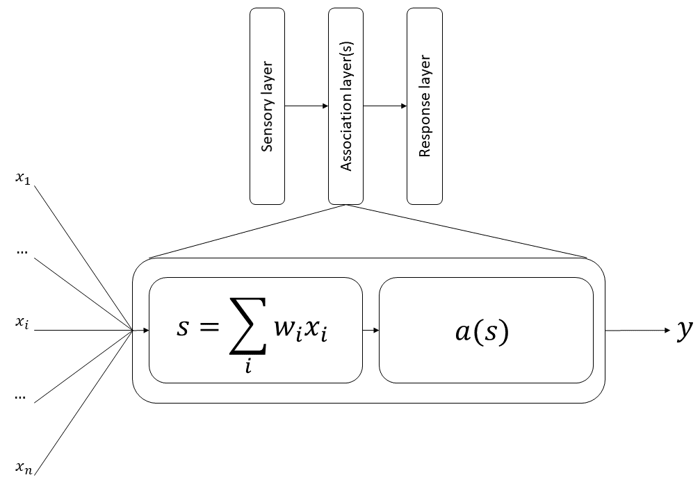
The next major step in the story comes in the late 1950s and early 1960s, with Frank Rosenblatt’s publications on the “perceptron” [58]–[60]. The perceptron was “a hypothetical nervous system (…) designed to illustrate some of the fundamental properties of intelligent systems in general” [58]. It should be noted that, while the term “perceptron” is sometimes used today to refer to a single artificial neuron [71], the “perceptron” in Rosenblatt’s publications is the entire network. Contrary to the very theoretical nature of McCulloch & Pitt’s work, Rosenblatt’s perceptron is also a physical machine. A 1957 technical report [59] describes the main components of the first version of the network: a sensory system (a set of photocells), a response system (lights which are lit up when their corresponding class is recognized), and an association system in between. Units in the sensory system have positive or negative connections to the association system. Each unit in the association system has a “fixed parameter” , “the threshold value which corresponds to the algebraic sum of input pulses necessary to evoke an output” [59]. This output is binary: the association units therefore perform a thresholding operation based on the input signal (see Figure 1.1). These units are then further connected to units in the response system, which “are activated when the mean or net value of the signals received exceeds a critical level.” The first perceptron had a single “association” layer, but Rosenblatt’s 1962 book [60] contains experiments on “multi-layer perceptrons,” containing several sequential association units. Different learning techniques are also discussed, including an “error-corrective reinforcement system” which changes the weights of the associations proportionnaly to the error made by the response unit, reproducing notions of learning introduced by Donald Hebb a few years earlier [1]. The conclusions from Rosenblatt’s work were very optimistic on the capabilities of the perceptron. While “single-layer” perceptrons (with one association layer) showed poor generalization capabilities, he noted that “the addition of a [second association] layer (…) permits the solution of generalization problems” [60].
In the late sixties, a big controversy arose around the perceptrons. The context of that controversy is well recapitulated in a Social Studies of Science paper by Mikel Olazaran [51]. The controversy opposed diverging views of Artificial Intelligence. The first one, exemplified by Rosenblatt, was trying to “build computational architectures bearing some resemblance to the brain’s nets of neurons.” Against this “connectionist” view were the proponents of “symbolic AI,” where the decision rules were encoded in explicit symbolic rules and algorithms. One of the leading researchers in that school of thought was Marvin Minsky. In 1969, Minsky and Seymour Papert published Perceptrons: An Introduction to Computational Geometry [48]. They focused on those single-layer perceptrons only, and set out to demonstrate that the limitations of perceptrons could not be overcome, and that further research in the domain was doomed to fail. The controversy lays mostly in the fairness of Minsky and Papert’s argument. As Olazaran notes, “strictly speaking, Minsky and Papert showed that single-layer nets, defined in a certain way, had some important limitations,” yet their stated conclusions went a lot further than that. Their version of the perceptron also had further constraints, for instance on the limit of incoming connections to a neuron, that did not exist in Rosenblatt’s work. Minsky and Papert’s book is often considered as the main cause of a rejection of neural networks in the late sixties, and the emergence of symbolic AI as “the only AI paradigm” [51]… for a time, and mostly in the United States and western Europe.
Minsky and Papert’s claim that multilayers perceptrons were essentially untrainable is disputed. Schmidhuber notes [65] that training mechanisms for multilayers perceptrons existed since the mid-sixties, and that “it seems surprising in hindsight that a book on the limitations of simple linear perceptrons with a single layer discouraged some researchers from further studying NNs.” Perhaps the most important contributor to neural networks during that time was Alexey Ivakhnenko. While he mostly published in Soviet journal “Avtomatika,”6 Ivakhnenko also summarized some of his work in English, as in a 1971 publication [29] where he presents an eight-layers perceptron trained with his “Group Method of Data Handling” (GMDH). GMDH networks are trained layer by layer, and use a validation set to “regularize” the network and remove unnecessary (“harmful”) units. Ivakhnenko also replaced the thresholding function used in the perceptron by a polynomial function.
1.1.3 Convolutional networks
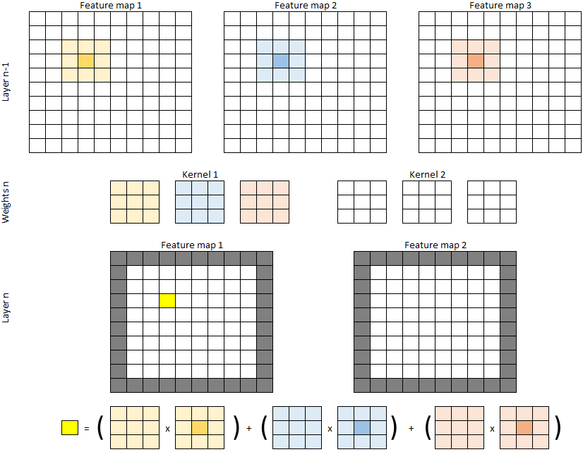
A big limitation of multilayers perceptrons is that the number of trainable parameters can get very large very fast, as the increase the number of neurons and thus of potential connections. A key development, particularly for computer vision, comes in 1980 with Kunihiko Fukushima’s Neocognitron [13]. The key ideas of the Neocognitron are to limit the connections in the network to a “receptive field,” which is a locally constrained subset of the neurons from the previous layer, and to share the weights of the connections between neurons of the same layer. While Fukushima does not use that particular vocabulary, this is essentially what is known as a convolutional network. A classical perceptron-like layer is fully-connected, or “dense.” This means that each neuron of layer is connected to each neuron of layer with an independent weight. If is the number of neurons in layer , a perceptron-like layer will therefore have learnable parameters. In a convolutional layer, the neurons will be organized so that their outputs form feature maps. Each feature map will be the result of the convolution between the input and a kernel (see Figure 1.2). If there are feature maps in layer and feature maps in layer , and each convolutional kernel has a size of , there will therefore be learnable parameters in the layer. The region in the input image which influences the value of a pixel of the feature maps of layer is called its receptive field. Each subsequent convolutional layer will therefore have a larger receptive field.
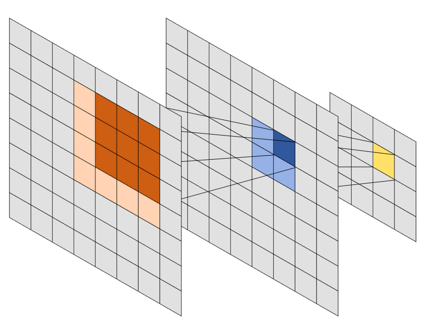
The other major contribution of Fukushima’s network is the idea of combining these “convolutional” layers with down-sampling layers, which reduce the size of the feature maps and, as a consequence, further increases the receptive field relative to the input image (see Figure 1.3). This idea is directly related to models of visual cortex and introduce an invariance to translation which is completely absent in perceptron-like architectures. A 32x32 pixels greyscale image connected to a 16x16 feature map using dense connections would take 262.144 parameters, while a convolutional layer with a 5x5 kernel would use only 25 parameters. Despite this enormous reduction in the complexity of the model, however, the performances of convolutional networks are excellent, as a “dense” network would need to essentially learn all patterns in all positions of the image independently, while a convolutional layer only has to learn them once.
Convolutional networks are thus particularly well-adapted to signals where there is a meaningful spatial relationship between the input elements, such as images. The “feature maps” produced by convolutional layers encode this spatial relationship in their structure. A layer that has 10 feature maps with dimensions of 25x25px thus encodes the response to 10 different kernels and the localisation of these responses.
1.1.4 Backpropagation and stochastic gradient descent
With the Neocognitron, we are getting a lot closer to something that would be recognized as a “deep neural network” today. If the “architecture” of the network is recognizable, the learning mechanism did not yet include what would become the standard for neural networks: backpropagation. Backpropagation appears to have been “discovered” (or at least applied to neural networks) independently by several researchers through the seventies and eighties, with the most often cited sources nowadays being Paul Werbos’ 1974 thesis [75] and David Rumelhart’s 1986 Nature publication alongside Hinton & Williams [61]. The history of the “invention” of backpropagation is subject to some amount of controversy. Jürgen Schmidhuber argued repeatedly, in his review [65] and in his personal online publications,7 that the credit for efficient backpropagation should go to the 1970 thesis of Linnainmaa, and that LeCun, Hinton and Bengio repeatedly failed to accurately reference his work, or the importance of Werbos’ work, in a bid to claim credit for themselves. Whether or not there are deontological problems with Rumelhart, Hinton & Williams’ work, it is clear that they wildly popularized backpropagation for neural networks. It should also be noted that neither Werbos’ work, nor especially Linnainmaa’s (who published his thesis in Finnish) had much visibility at the time, and that it is entirely plausible that Rumelhart and Hinton had not read any of their contributions. The ongoing feud between Schmidhuber and Hinton, spanning their academic works, social network publications8 and blog post responses9 demonstrates how difficult it is to get an accurate, unbiased historical record.
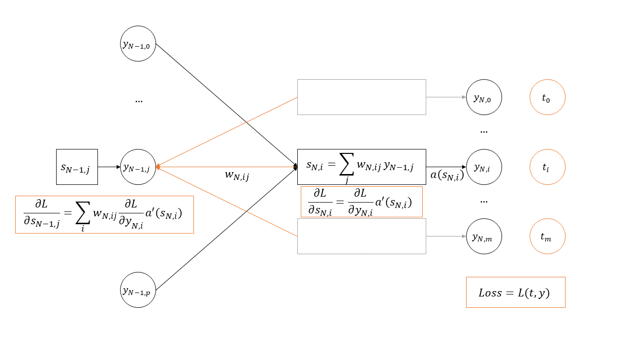
Backpropagation is a way to implement gradient descent to optimize the weights of a multilayers neural network in order to minimize an error function (usually called the loss function in modern terminology), as illustrated in Figure 1.4.
Let be the target output of a network, an input vector, and the output of the network with representing all the connection weights within the network. The loss, in general, is a function of and (which could be vectors or scalars depending on the problem):
With gradient descent, the goal is to compute the gradient of the loss function with regards to the weights:
So that the weights can be updated using a certain learning rate :
The problem that backpropagation aims to solve is that cannot be computed directly, and so gradient descent alone cannot be used to update all the weights of the network. Backpropagation starts from the last layer of the network:
Where is the number of layers in the network, is the output of the -th neuron of the -th layer, and is the weight of the connection between the -th neuron of the -th layer and the -th neuron of the -th layer. It should be noted that in many formulations of the operations happening at the neuron level, there will be an added bias term to the summation. However, the complete formulation is equivalent to the formulation presented above if we simply consider that the bias is associated with a constant input of 1.
The first step is to compute the derivative of L with respect to $s_{N,i}, which using the chain-rule of partial derivatives gives us:
With the total derivative of the activation function.
If the loss function was chosen to be derivable with respect to , all the terms of this equation can be directly computed. For instance, if the loss function is the mean squared error:
With the number of output neurons of the network, then .
The next step is to propagate the error to the previous layers, using the rule:
This allows for the computation of in every neuron of the network. From there, the gradient relative to the weights can also be computed:
Each weight can then be updated with:
While the error can be computed on the entire training set before updating the weights, a stochastic gradient descent method was quickly preferred, updating the weights based on a single example at a time (or a small “mini-batch”), for better convergence speed. This was notably discussed by Yann LeCun and several colleagues in 1989, presenting a convolutional network using backpropagation to recognize handwritten zip codes for the U.S. Postal Service [39].
LeCun’s publications on handwritten digits and, later, document recognition [37], [39], [41] may be a turning point in neural networks, not so much because of the novelty of any specific part of his methods, but because of its very practical aspect. They showed that convolutional neural networks, trained with stochastic gradient descent and backpropagation, using sigmoid activation functions, could be trained to solve practical, real-world computer vision problems. LeCun’s 1998 “LeNet-5” has all the characteristics of a standard classification architecture, as seen in modern deep learning models: a succession of convolution and down-sampling (with max-pooling) layers which increase the number of feature maps while decreasing their size, followed by a few “dense,” perceptron-like layers with decreasing number of neurons until the last output layer, which contains as many neurons as there are classes to discriminate.
1.1.5 The vanishing gradient and “deep” improvements
The main issue that neural networks faced in order to go “deeper” was the “vanishing gradient” problem, formally described by Sepp Hochreiter in his 1991 Ph.D. thesis in German and published by Hochreiter and Schmidhuber in 1997 [25]. The vanishing gradient problem is a direct consequence of the backpropagation algorithm. As the “gradients” are propagated through the network, the derivatives of each layer’s activation functions are multiplied together. The most common activation functions at the time were sigmoid functions such as the logistic function or the hyperbolic tangent (shown in Figure 1.5). The derivatives of these functions have a small peak in the centre, and quickly fall close to zero on both sides. This has a catastrophic effect on learning, as the multiplication of those very small gradients lead to some weights in the network being essentially incapable of being updated.
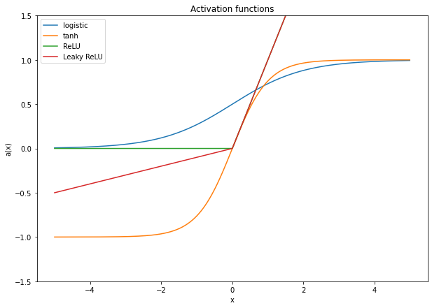
Some improvements were proposed to address this problem over the next years. Hochreiter and Schmidhuber’s Long Short-Term Memory for recurrent neural networks was explicitly designed to avoid vanishing gradients [25]. Changing the activation function to the Rectified Linear Units (ReLU) [50] and its variations such as Leaky ReLU [45] (see Figure 1.5), which have a much larger “active” region (in the sense of a range of input with a significantly larger than zero output), also proved to be very effective. The “old” idea of training a network layer-by-layer was also one of the key ideas of Hinton’s 2006 “deep belief” article [23], which also used an “unsupervised” pre-training step. As we have mentioned at the beginning of this section, this publication is when the terms “deep learning” and “deep neural network” start to gain traction. “Short-skip” and “long-skip” connections, such as in Highway Networks [70], ResNet [22] and U-Net [57], which create bypasses through which the gradients can flow more easily to early layers also helped to overcome the limitations of deeper neural networks.
1.1.6 The Deep Learning revolution
As we mentioned at the beginning of this story, a key year for the deep learning revolution was 2012. Yet none of the networks or learning methods that cemented themselves as the state of the art of computer vision at that time were very different from anything that existed before. In fact, as we have seen through this historical review, all the major elements of “deep learning” publications slowly evolved in incremental steps, building on top of each other.
Is “deep learning” therefore really a buzzword, a rebranding of neural networks? There is no doubt that some form of revolution happened, but it was obviously not a revolution in the core theory of neural networks. Two major contributing events, however, can be traced to the same period. The first is the start of the “Big Data” era [63]. All these 2012 works relied on datasets of sizes and diversities which were simply unimaginable a few years earlier. ImageNet and Google’s databases in particular use millions of diverse colour images. MNIST, LeCun’s 1998 database of handwritten digits, had by comparison 60.000 small, aligned, black-and-white images, which were resized to 28x28px (with interpolated values, so that the final images are greyscale [39]).
The second event was the massive development of general computing on graphical processing units (GPU). In 2006, the release of CUDA by NVIDIA made parallel processing on GPUs a lot more accessible by allowing developers to use C to program GPUs [74]. As neural networks are massively parallelizable, it was quickly shown that training neural networks on GPUs causes massive speedups in training time, thus allowing larger networks to be trained [54].
The deep learning revolution therefore appears to be more of a practical than theoretical one. As “Big Data” provided the amount of training samples required for training networks with large number of parameters without massive overfitting and GPUs made the training times more reasonable, large neural networks suddenly became something that could realistically be done outside of hyper specialized research groups with access to supercomputers.
This, in turn, led to the release of software tools designed to make the building and training of large neural networks easier and even more accessible. Starting from 2009, Theano was developed at the University of Montréal , providing a Python framework for fast tensor operations on GPUs [6]. Other frameworks such as Caffe, developed by Berkeley AI Research and released in 2014 [30]; TensorFlow, released by Google in 2015 [2]; or Facebook’s PyTorch, presented at NeurIPS 2019 [52]; contributed to the widespread adoption of deep neural networks outside of pure machine learning research and into practical applications.
This practicality also shows that the study of neural network did not only evolve in its theory, but also in the objectives of its actors. Early connectionists were overtly interested in using machine intelligence as a proxy for better understanding human intelligence, and the process of learning. We then see a movement towards studying machine intelligence by itself: artificial neural networks did not necessarily have to resemble animal neural networks anymore, the main concern was that they were capable of learning ever more complex functions. Finally, we get to the modern vision of task-oriented deep learning, exemplified by the importance that “Grand Challenges,” benchmarks and competitions have taken in the deep learning era.
1.2 Defining deep learning
From this historical perspective, it is clear that the concepts of artificial intelligence and its subdivisions have fluctuated over time. Definitions of “artificial intelligence,” “machine learning,” “deep learning” and all related concepts can vary in the scope of what they include. In this section, we will provide and justify the definitions that will be used in the rest of this thesis.
– Artificial intelligence is the study of systems which take actions or make decisions based on their perception of their environment.
This is a very broad definition. A key part is that artificial intelligence systems do not exist in a vacuum: they perceive and act on the “real world,” and both the perception mechanism and the action/decision mechanism are a part of that whole system. In computer vision, the “perception” would typically be some form of image acquisition, and the “action” could be, for instance, the generation of semantic information extracted from the image.
– Machine learning is the study of artificial intelligence systems that are capable of improving their performance based on their experience.
This implies two very important aspects of a machine learning agents: they must include parameters that can be changed as a response to the observations, and they must include a metric for measuring its performance, as well as a mechanism for updating its parameters. These are determined by the machine learning model and the machine learning algorithm:
– A machine learning model describes the relationship between the input of the system (the “perception”) and its output (the “action”), as well as the parameters of that relationship. When the parameters are set, the model is said to be trained.
– A machine learning algorithm is a method used to find the best parameters of the model according to certain criteria.
Machine learning problems are often separated into “supervised” and “unsupervised” problems:
– A supervised problem is one where each sample in the training set is associated with a known target value (the “label”).
– In an unsupervised problem, the labels in the training set are unknown, and the model has to learn from the distribution of the data.
A useful distinction can also be made between the “parameters” and the “hyper-parameters” of a model.
– The parameters are internal to the model and are set through the learning algorithm.
– The hyper-parameters are external to the model and are often set through the validation process. They are typically related to design choices in the model, like the maximum depth of a decision tree, or the size of the layers in a convolutional neural network.
It is often the case that a machine learning model can be split into two parts: feature extraction and decision function.
– Features extraction is a processing of the raw input of the system to project it into a new space of variables (the “features space”) where the problem is easier to solve.
– The decision function is a mathematical relationship between the input in features space and the output of the system.
A further distinction is made in the features extraction step depending on how those features are determined:
– Handcrafted features are chosen and defined by a human expert based on their experience and their observation of the data.
– Learned features are derived from the data by a machine learning algorithm. The subset of machine learning that include learned features is called representation learning.
We can now finally arrive at the elements that separate so-called “deep” learning from the rest of machine learning:
– Deep learning is the study of machine learning models where features are represented in a layered structure of increasing abstraction, and of machine learning algorithms that learn the features representation and the decision function as a single step.
From this definition, we get the key aspects of what would generally be described as a “deep learning” system today.
Layers of abstraction: low-level features are extracted from the raw input of the system, and higher-level features are learned by combining these low-level features.
Learning features and decision in one step: the main difficulties that prevented multi-layered neural networks to learn efficiently in the past were generally related to the ability to efficiently learn the layers further from the output. Solutions to that problem typically involved learning layer-by-layer, but that effectively means learning the features representation separately from the decision function, which falls into the broad category of “representation learning” without being really specific to deep learning.
This definition also implies that the answer to the question of whether, for instance, perceptrons of the past belong to the “deep learning” category actually depends on how they were used and trained. The original, single-layer perceptron of Rosenblatt was trained directly on the raw input, and learned “features” and “decision” in one step, but it clearly did not include layers of abstraction. A multilayers perceptron could be included in the “deep learning” category if applied directly on the raw data, but not if it relied on handcrafted features. The perceptron-like networks of Ivakhnenko, for instance, were trained layer-by-layer and relied on handcrafted features in the examples he used [29], and would not be included either. Fukushima’s Neocognitron [13] is much closer to the definition, as it clearly demonstrates layers of abstraction and learn directly from pixel data, yet the images used are synthetic, binary representations of numbers and letters, and the network is trained in an unsupervised way and does not include any “action” step. The letters or numbers are not classified: it is just observed that the network has learned different responses to different types of patterns. LeCun’s handwritten digits recognition [37] includes a big pre-processing step to isolate the digits and standardize their presentation, yet its inputs are still close enough to the raw data that it is probably reasonable to include it into the “deep learning” definition. As a direct predecessor to the highly publicized AlexNet [36], it is also unsurprising that it represents one of the common archetypes of modern deep neural networks for computer vision: the “image classification” network.
This definition of deep learning does not necessarily require the model to be any type of neural network. However, in practice, most if not all model used in modern deep learning are neural networks, making “deep learning model” and “deep neural networks” functionally synonyms. It is therefore useful here to also introduce a few definitions relative to neural networks.
– An artificial neural network (generally just shortened to “neural network” in the context of machine learning) is a model that can be decomposed into a graph of interconnected units (the “neurons”) which perform a weighted sum of their inputs, with an activation function that may introduce non-linearities in the overall function. The structure of the graph is often referred to as the architecture of the network.
While it is in theory possible to explicitly model every single connection and every single neuron in a network, it is generally more practical to use an organization in layers:
– A layer in a neural network is a group of neurons that share a common set of inputs and outputs and no “internal” connections (as in: no neuron in the layer is connected to another neuron in the same layer). Neurons in a layer will also typically share the same activation function.
– A connection exists between layers if the output of some neurons of one layer are used as input by some neurons of the other.
Finally, it is sometimes useful to be able to refer to multiple functionally related layers at the same time. We will refer to those groups of layers as blocks:
– A block is a group of layers in a neural network that perform a particular function together within the network.
1.3 Computer vision tasks
A complete taxonomy of computer vision tasks is outside of the scope of this thesis, but we will in this section propose a useful framework for categorizing the different types of tasks that will be relevant to the rest of this work.
First, what do we mean by a “Task?” To quote Goodfellow et al: “Machine learning tasks are usually described in terms of how the machine learning system should process an example.” [16] In other words, a Task is defined by the type of output that is expected, and the kind of input that is being processed. In computer vision, the input will typically be an image, most likely represented as a matrix containing the pixel values. It should be noted that with this definition we are not considering differences in the learning process (for instance: supervised or unsupervised learning), which can lead to completely different categorizations of machine learning algorithms.
One big distinction that can be made relates to the nature of the output value. In classification tasks, the desired output comes from a discrete, finite set of possibilities. In regression tasks, the output consists in a set of continuous variables [7].
For most of the tasks that we are concerned with in this work, however, a more useful categorization is related to the nature of the target: the images, objects, or pixels.
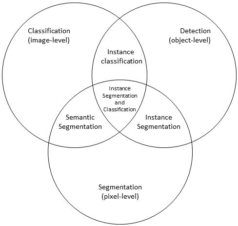
– In a classification task, the goal is to assign a class to an entire image. The output of such a task will typically be a single class, often supported by a vector of class probabilities. In some cases, the categories can be ordered.
– In a detection task, the goal is to detect the presence of instances of a target object. The output of such a task will typically take the form of a set of bounding boxes within which the instances have been found.
– In a segmentation task, the goal is to separate the “foreground” pixels (which are parts of “objects of interest”) from the “background” pixels (everything else). The output will take the form of a binary mask, often supported by a pixel probability “heat map.”
These three basic tasks can be combined with each other to form more complex tasks:
– An instance classification task combines object detection with classification (assign a class to each of the detected objects). The output will typically be a set of bounding boxes with corresponding class values (supported by vectors of class probabilities).
– An instance segmentation task combines object detection with segmentation (determine which pixels are part of which object instance). The output will be a pixel “label map,” where each pixel is assigned to a label representing the object that it belongs to.
– A semantic segmentation task combines pixel segmentation with classification (assign a class to each of the pixels). The output will be a pixel “class map,” often supported by a “class probabilities” map where each pixel is associated to a vector of class probabilities.
– An instance segmentation and classification task combines all three basic tasks, so that each object is detected, assigned to a class, and associated to a pixel mask. The output will be a class map alongside a label map, or a label map with an associated “per-label” class prediction.
It should be noted that, while regression tasks are not explicitly represented in that categorization, they will generally be very close to one of these (except that class values will be replaced by continuous values). For instance, a counterpart to “semantic segmentation” could be “image generation,” where for each pixel a colour value is predicted. This categorization is also not exhaustive. Image registration, for instance, does not really fit into this taxonomy. These however cover the tasks where deep learning methods have been most relevant in digital pathology and will be where we will focus our attention in this work. For the same reason, we will generally limit ourselves to supervised methods, and only consider “unsupervised learning” as a pre-training step (as in representation learning) in the context of a supervised task.
1.4 The deep learning pipeline
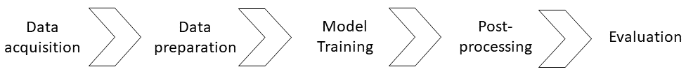
While the nature of the different tasks will certainly also influence the design of the learning process, most machine learning solutions to computer vision problems will follow a relatively similar pipeline, illustrated in Figure 1.7. Deep learning solutions follow the same process. Each of the steps in this pipeline come with their own challenges and are largely application dependent. In this section, we will briefly explain the elements that are commonly found in computer vision pipelines. A summary of the hyper-parameters that are related to these different steps is presented in Table 1.2.
| Hyper-parameter | Choices and possibilities |
|---|---|
| Pre-processing steps | Resizing, tiling, colour space change, de-noising… |
| Data augmentation steps | Affine/elastic transforms, noise, blur, colour transforms, GANs… |
| Mini-batch size | Trade-off between memory availability, training speed (larger size = quicker) and end result quality (smaller size may be better). |
| Initializer | Xavier [15], He [21]… |
| Optimizer | Adam [26], RMSProp [24], ADADELTA [80]… |
| Loss function | Cross-entropy, mean-squared error, customized losses… |
| Stopping criterion | Fixed number of epochs or based on improvement on a validation set. |
| Post-processing steps | Image reconstruction, resizing, de-noising, labelling… |
| Evaluation process | Metric, aggregation method, statistical tests… |
1.4.1 Data acquisition
The data acquisition step will obviously be largely concerned with the technical aspects of the acquisition. For instance, in digital pathology, the variety of protocols that were applied for processing and staining the tissue samples and the scanners used to acquire the images will influence the final result. It is also concerned with the selection of the samples. A machine learning algorithm will learn to use the data that is provided in the training set. If this data is not representative of the domain of applicability, the algorithm will most certainly fail.
Another closely related question is the constitution of the training set and of the test set (and/or the validation set). The training set is the data that is used to determine the learnable parameters of the model. The validation set is used to determine the hyper-parameters of the model and of the algorithm. The test set is used to evaluate the model once all parameters and hyper-parameters have been fixed. Improper handling of the data can lead to bad interpretation of the results. As a general rule, the test set should be as “independent” from the training and validation set as possible: different acquisition hardware, different sample source (e.g., individual patients in a medical application), etc. More independence means that the test set evaluation will more accurately represent the generalization capabilities of the algorithm.
Equally important to the supervised learning process as the image acquisition is the annotation of the data. The ideal situation for a deep learning algorithm is to have a perfectly supervised dataset, meaning that to each data sample is attached a “ground truth,” which is the expected output of the trained algorithm for that sample. This optimal situation is rarely found, particularly in digital pathology datasets. This will be discussed at length in the rest of this thesis.
1.4.2 Data preparation
Even “deep learning” algorithms can usually not simply take as input the whole training set. Some pre-processing will typically be necessary. The pre-processing that needs to be applied will again depend on the application. Two distinct types of pre-processing are very common in computer vision application: normative pre-processing and data augmentation.
Normative pre-processing includes steps designed to restrict the domain of the input space. For instance, many network architectures require a fixed-size input. Pre-processing steps to achieve that include resizing or tiling of the input images. It may also be interesting to change the colour space (for instance, moving from RGB to HSV, or to a colour space more relevant to the application). A normalization of the dataset can also be done at this stage, or a rescaling of the input values to a predetermined range (for instance, -1 to +1).
Data augmentation has a very different role. It seeks to increase the size and diversity of the dataset by generating artificial examples based on the available samples. Instead of restricting the domain of the input space, the goal is in this case to fill this domain with as many (realistic) examples as possible. Common data augmentation steps include affine transforms, blur, noise, colour transforms, elastic transforms, etc. GANs can also be used to generate new examples (although this solution sometimes just deports the problem of finding real examples to the training of the GAN itself).
1.4.3 Training of a deep learning model
While training the model, data samples are generally presented in batches (often referred to as “mini-batches”), with the parameters of the network being updated after each batch. The batch size is a design choice that is often constrained by the available hardware, as using larger batches require more memory usage in the GPU. At the extreme end of the spectrum, training can be done with batches consisting of a single example. This is for instance the case in stochastic gradient descent. The batch size can influence both the speed of the training process, and the quality of the results. As a general rule, larger mini-batches tend to train faster, but lead to worse generalization [33], [43], [46].
When training neural networks from scratch, another important aspect is the initialization of the parameters. The initial parameters of the connections are chosen randomly, but the choice of distribution from which these random weights are drawn is important, as bad initialization can lead to a higher risk of vanishing or exploding gradients [19]. Usual choices are to use either a normal or a uniform distribution, with a mean of 0 and a variance that depends on the number of neurons in the layers on both side of the connection. The two most common variants are Xavier initialization [15] and He initialization [21]. Xavier initialization was initially designed for networks using the tanh activation function, while He initialization was designed to adapt it to networks using the “rectified linear units” (ReLU) functions.
Another important aspect of the learning algorithm is the choice of the optimizer. All commonly used optimization techniques for deep neural networks are based on gradient descent and backpropagation. The main steps of this optimization process are:
- Computing a loss L on a mini-batch, which measures the error that the model currently makes on the training data.
- Use the rules of backpropagation to compute the contributions of each parameter w of the model to that loss: .
- Update the parameters depending on their contribution to the loss and to a learning rate :
The learning rate can be fixed through the learning process or can be adaptive. More than a hundred different optimization methods have been proposed for training deep neural networks, but no clear rule has emerged to determine which one should be used for a particular problem, with some research suggesting that the difference between methods is often less important than the difference that can be observer within the same method with different hyper-parameters or even with different random seeds [66].
The result of those optimizers will also obviously depend on the loss function being used. The default, general purpose loss functions are the cross-entropy (CE) for classification problems and the mean-squared error (MSE) for regression problems, defined as:
With the number of samples, the number of classes, the binary target value of sample for class (for classification problems), the scalar target value of sample (for regression problems), and with and similarly defined for the output of the model.
More complex loss functions can be used to address problems such as class imbalance [44] or noisy labels [31].
Finally, another choice that needs to be made is the stopping criterion for the optimization process. The simplest rule is to run the optimizer for a fixed number of epochs (one epoch meaning that all training samples have been processed once), but this can easily lead to over-fitting. Early stopping is a common choice to avoid this problem, with a stopping rule that uses the validation set to check if the learning has failed to improve by more than a certain threshold value for more than a certain number of epochs (the “patience”).
1.4.4 Post-processing
After the optimization process is complete, the output of the model may not be completely usable as such yet. For instance, in a segmentation problem, if the pre-processing step included a tiling of the image, the output of the model will also be tiled, whereas the true target output for the whole pipeline is a segmentation of the full image. Image reconstruction from the segmented tiles may therefore be necessary as a post-processing step. If the tiling was done with some overlap, the reconstruction rule is not trivial, as individual pixels will have different predicted values when they are included in multiple tiles. Their final output value may be determined as the average of the predicted probability values, but other rules may also be applied such as the maximum value, or a weighted average with the weight depending on the proximity to the centre of the tile (as predictions will tend to be better further from the borders).
Other post-processing steps may include some de-noising (for instance, using morphological operations to remove isolated predicted pixels and to smooth the borders of segmented objects), or labelling (in the case of instance segmentation).
1.4.5 Evaluation
The evaluation of a deep learning algorithm is a very important aspect of the process, as it is used not only to determine which model and which set of hyper-parameters are best for solving a particular task, but also to validate if the end results are adequate for a certain purpose (such as a clinical application).
We have previously mentioned the selection of the test set as an important aspect of the data acquisition process. It will of course also influence the quality of the evaluation. The most obvious aspect of the evaluation is the metric used. The choice of a good metric is important as different metrics will be associated with different biases.
Different metric aggregation methods can be used. The metric can be computed on every image of the test set, then averaged using the mean or the median. It may also be possible (for instance in segmentation problems) to compute the metric on the whole test set at once (giving more impact to larger images), or to first aggregate according to some sub-groups (for instance: per-class in a multi-class problem, per-patient, etc.)
In addition to this “averaged” value, it is often useful to look at the distribution of the metric over the test set. This allows for a more robust analysis, using for instance statistical tests to assess the significance of the results when comparing different algorithms, or different sets of hyper-parameters.
1.5 Deep model architectures
If your task is similar to another task that has been studied extensively, you will probably do well by first copying the model and algorithm that is already known to perform best on the previously studied task.
Goodfellow, Bengio & Courville; Deep Learning, 2016 [16]
There is an infinite number of possibilities when defining the architecture of a deep neural network. Many practically used networks, however, share a lot of common characteristics and are made from the same building blocks. In this section, we will look at these building blocks, and how they are integrated into the architectural “archetypes” used in many computer vision tasks. We will not look outside of computer vision, as these are the type of applications most relevant to digital pathology. We will therefore not cover recurrent neural networks or LSTMs [25], commonly found in domains with sequential signals such as Natural Language Processing.
We can look at deep learning architectures at different levels. At the “macro” level, we have the overall “shape” of the network, which is mostly dependent on the inputs and outputs of the system (in other words: on the task). At the “micro” level, we have smaller design choices in which specific layers are used, and how exactly they are connected.
We will first look at the most common types of layers used in deep neural networks, then we will move on to the macro-architectures in relation to the tasks defined previously, and finally look at some of the micro-architectural choices and how they can affect the learning process and the performances of the model.
1.5.1 Layers
Dense (or “fully-connected”) layers are the simplest layers from a conceptual point of view. The n-th layer of a network is dense if every neuron in layer n-1 is connected to every neuron in layer n. Mathematically, dense layers are very easy to model using matrix notations:
Where is a vector containing all the outputs of the -th layer, is a matrix containing all the weights between each neuron of the -th layer and each neuron of the previous layer, and is the activation function of the -th layer. The main role of dense layers in modern convolutional networks is to perform the discrimination step based on the learned features, in a classification task. The number of learnable parameters in a dense layer depends on the number of neurons of the layer and of the previous one. If dense layer has neuron, and layer has neurons, there will be learnable parameters in the layer.
Convolutional layers are very common in computer vision applications. One of their key characteristics is that they keep a sense of spatial relationship between the neurons. Neurons in convolutional layers are organized so that their outputs form “feature maps,” which are essentially images that are the result of a convolution between the feature maps of the previous layers (or the input image) and some convolutional kernels. These kernels are small, usually square matrices (see Figure 1.2) whose values are the learnable parameters of the layer. The number of learnable parameters in such a layer therefore depends on the number of feature maps and the size of the convolutional kernels. If layer has feature maps, layer has feature maps, and the convolutional kernels are squares, there will be learnable parameters.
Pooling layers, as mentioned above, are very often found in combination with convolutional layers in networks designed for computer vision. Pooling layers do not have any learnable parameters. Like convolutional layers, they depend on the spatial relationship of the neurons in the previous layer, and they usually compute a simple statistic (often the maximum, but sometimes the mean or the median) on neighbourhoods. While “max-pooling” and “average-pooling” are the more common options, other variants have been proposed (such as probabilistic approaches which introduce some randomness in the pooling) [3]. They serve as a down-sampling step so as to increase the receptive field of the next layers, and, when using max-pooling, as a way to focus the attention of the network on the neurons that are active for a particular input (see Figure 1.3).
Up-sampling layers are used to increase the resolution, as a sort of “inverse” step from the pooling layers. Different techniques can be used for the up-sampling, including interpolation [57], transposed convolution [79], and methods using the pooling indices of the down-sampling layers to take into account the position of the feature map’s pixels in the original image [5].
Regularization layers can be used to reduce the risk of overfitting and to increase the convergence speed of the learning process. The two most common options are “dropout” [69] and “batch normalization” [28]. Dropout works by randomly filtering out the signal between two layers during training (setting the weights of a fraction of the connexions to 0). This will force the network to learn redundant pathways for encoding distinct features, encouraging a better generalization capability. Batch normalization consists in re-scaling and re-centring the inputs of a layer based on the distribution of a mini-batch [28]. During the training phase, a running average of the mean and standard deviation on the whole training set are also computed and can be used for “normalizing” new samples on the trained network.
1.5.2 Macro-architectures: how networks adapt to tasks
A common way of looking at deep neural networks is to separate them into two parts: a “general purpose” feature extraction part, sometimes called the encoder, and a “task specific” part that will combine the features to arrive at the desired output. This, of course, makes it easy to relate deep learning methods to “classical” machine learning, where the “feature extraction” part would use handcrafted features.
The distinction, in a deep neural network, is however somewhat arbitrary, as all layers are typically trained together to both extract features and perform the task. The distinction, however, does make sense from a macro-architectural standpoint, as almost all computer vision models start with a relatively similar encoder.
The encoder is mostly made of a succession of convolutional layers and of pooling layers. At the end of the encoder, we will generally find a large amount of “feature maps” with a very low resolution. What comes after the encoder largely depends on the type of task that the model is designed to solve.
Classification tasks require an image-level class probability vector as the output. The associated macro-architecture will be to follow the encoder with a “discriminator,” which is made of several successive dense layers like in a standard multilayer perceptron.
Detection tasks where the target outputs are bounding boxes are equivalent to binary classification tasks on the sub-image contained within those bounding boxes. Detection models therefore typically combine a “region proposal” part with a classification network. The encoder will often be trained on the full images, then another process (which can be another neural network) will produce candidate regions of interest, and a discriminator will be trained on those regions of interest to identify those that include the target object.
Segmentation tasks require a per-pixel prediction. The most common way of achieving that is to follow the “encoder” with a symmetrical “decoder.” A decoder is made of a succession of convolutional layers and up-sampling layers. Starting from the low-resolution feature maps at the end of the encoder, it will produce a high-resolution output.
Some of the extensions to the more “complex” tasks are straightforward. For instance, the difference between “simple” binary segmentation and “semantic segmentation” can simply be the number of output channels in the decoder. Similarly, instance classification just implies having a multi-class discriminator in the detection network.
The case of instance segmentation is more complex, with two distinct approaches commonly used. The first one is based on the “detection” networks and adds a branch to the network which is trained as a decoder to produce a segmentation on a detected region of interest. In this case, “instance segmentation” is therefore seen as “instance detection, with segmentation.” The other approach starts from the segmentation, and then tries to separate the potentially overlapping instances. These networks will therefore generally have an encoder, followed by one or several decoders (for instance, one trained to segment the objects themselves, and the other specifically trained to segment the “borders”), and a post-processing step (usually outside of the neural network) that will take the outputs of the decoders and compute the label map. Instance segmentation and classification can be achieved by extending any of these approaches to a multi-class case.
Two others commonly found architectures that may be useful to introduce here are the auto-encoder architectures (which can be used for instance for unsupervised feature extraction) and the Generative Adversarial Networks (GAN), which can be used for image generation problems such as super-resolution [4].
Auto-encoders follow the same basic architecture as the segmentation network, with an encoder and a decoder block. The key difference is the output: instead of class probabilities, the output will be pixel values, and the auto-encoder will be trained to reconstruct the input image (so the target output is the same as the input).
An auto-encoder will therefore learn sets of features that best characterize the images present in the dataset in a way that is independent of any further usage of the data. On its own, such a network can be useful for applications such as image compression [10], noise filtering [42], anomaly detection [72] or super-resolution [35]. It can also serve as a first step in a semi-supervised learning strategy [12], learning the feature representation with an auto-encoder and then using those features as a pre-training on a supervised dataset.
Generative Adversarial Networks (GAN) combine two different networks with separate goals: a “generator,” which learns to produce realistic data, and a “discriminator,” which learns to detect if a data sample is “true” (meaning that it comes from the real dataset) or “fabricated” by the generator [17].
The generator will typically take the same architecture as a “segmentation” network, with an encoder block and a decoder block. The key difference is that the input of the generator will be random noise, and its output will eventually be a realistic image. The discriminator, on the other hand, will be a classification network.
A summary of these task-adapted macro-architectures is presented in Table 1.3.
| Task | Macro-architecture(s) | Example network(s) |
|---|---|---|
| Classification | Encoder + Discriminator | AlexNet [36], DanNet [11] |
| Detection | Encoder + Region Proposal + Discriminator | Fast R-CNN [14], YOLO [56] |
| Segmentation | Encoder + Decoder | U-Net [57], SegNet [5] |
| Instance segmentation (and classification) | Encoder + Region Proposal + Discriminator + Decoder | Mask R-CNN [20] |
| – | Encoder + Decoder(s) + Post-processing | DCAN [9], HoVer-Net [18] |
| Others | Auto-Encoder, GANs | MCAE [49], DCGAN [53] |
1.5.3 Micro-architectures: infinite choices
While most deep neural network architectures have very similar macro-architectures, infinite variations appear as soon as we look into the finer details of the model. These variations are where most of the “hyper-parameters” of the network itself can be found. In this section, we will briefly explain the most important choices that need to be made in the design of a network at the micro-architectural level. A summary is presented in Table 1.4.
| Hyper-parameter | Choices and possibilities |
|---|---|
| Depth (number of layers) | Trade-off between the capacity for higher levels of abstraction and the risks of overfitting and difficulties in learning. |
| Width (number of kernels / feature maps) | Trade-off between capacity for learning more features and the risks of overfitting and longer learning time. |
| Size of convolutional kernels | Variable effect on training time and performance. |
| Size of pooling (and un-pooling) layers | Larger pooling increases the receptive field faster through the layers but loses more information along the way. |
| Activation functions | Most recent models use variations of the ReLU function [50]. |
| Residual units’ usage and structure | If “short-skip” connections are used, number of convolutional layers skipped and concatenation method. |
| Dropout parameters | Dropout layers may be put at different parts of the architecture for regularization, with as a hyper-parameter the percentage of connections to randomly set to zero during training. |
| Use of Batch Normalization | Should “batch normalization” layers be introduced in the network for regularization? |
| Long-skip connections | Choice of which low-level features to re-introduce in which later stage of the network. |
| Order of the layers | Number of convolutional layers, of pooling layers, position of the regularization layers, etc. |
- Network depth: the depth of the network is controlled by the number of layers between the input and the output. For encoders, decoders, and discriminators, there could be any number of convolutional layers, dense layers, pooling and un-pooling layers. In general, deeper networks have a higher capacity for “abstraction,” but require more resources to be trained and have a higher risk of overfitting.
- Number of kernels (and associated feature maps) for each convolutional layer. This is often referred to as the width of the layers. A common trend is to increase the number of feature maps as we progress in the encoder (and reduce the size through pooling), and to decrease the number of feature maps through the decoder. The same choice needs to be made with the number of neurons in dense layers, which will also typically start large and then be reduced to eventually match the number of classes at the output.
- Kernel size and pooling size. In convolutional layers, the size of the kernels will determine the number of trainable parameters of the model. The choice in general is to either have fewer convolutional layers with larger kernel sizes, or to stack more convolutional layers with smaller kernels (with 3x3 kernels a very common choice). For pooling, larger sizes mean that the receptive field of the feature maps increase faster, but more information is lost in the process. The effect of these choices can be very different depending on the network, application, dataset and training algorithm, and there are no hard rules on what the “best” choices are.
- Activation functions. Convolutional and dense layers typically involve a two-steps computation, with first a linear operation on their input (the weighted sum) followed by an activation function. In “older” neural networks, sigmoid functions such as the logistic function or the hyperbolic tangent were often used, but since the introduction of “Rectified Linear Units” [50], ReLU and its variants such as “Leaky ReLU” [45] have been the most widely used (see Figure 1.5).
- Residual units or residual blocks are the most common example of “short-skip” connections. The principle of a residual block is to create a branching in the network, such that one branch goes through a series of convolutional layers, and the other branch takes a shortcut and is fed back into the result of these convolutions (see Figure 1.8). In the original ResNet [22], the “convolutional” path includes two convolutional layers, while the “shortcut” path is a simple identity mapping, and the two branches are merged with an addition. Many variations on this idea exist [78]. The number of convolutions in the convolutional path may vary, and there can be more than two branches. Using the addition operation at the end requires that the shape after the last convolution is exactly the same as the shape of the input. This means either having the same number of feature maps in the last convolution as in the input or adding a single convolution in the “shortcut” path. Alternatively, the addition can be replaced with a “concatenation” so that the two paths may have a different number of feature maps. Residual units largely mitigate the vanishing gradient problem by allowing the gradients to flow through the “shortcut” during backpropagation, thus making the training of deeper networks possible.
- Regularization parameters. Whenever regularization layers are used, they come with their own set of choices and parameters. The position of the dropout or batch normalization layers in the overall architecture, and the number of such layers, can be changed. In a dropout layer, the percentage of dropped connections during the training phase also has to be set.
- Long-skip connections are another type of shortcuts in the network architecture. Their main goal is to re-introduce high resolution features to layers in later parts of the network, particularly in the decoder of segmentation networks, which without the skip connection would only see heavily down-sampled feature maps. Where exactly those skip connections should be placed is another micro-architectural choice that needs to be made.
- Order of the layers. While the overall shape of the architecture is dictated by the macro-architecture and generally related to the task definition, there are still smaller-scale choices to be made in the exact ordering of the layers: how many convolutional layers should be placed in between pooling layers? How many pooling layers should there be?

1.6 Lost in a hyper-parametric world
Beyond the constraints of the task to be solved, the choices to be made while designing a deep learning solution to a given problem create an essentially infinite hyper-parameters space (and it could be argued that the definition of the task itself is a hyper-parameter of its own, as the translation from the “real-world” objectives to a formal definition is not trivial).
The question on how to best optimize all these hyper-parameters is still widely open. Automated methods have been proposed, using Bayesian optimisation [81] or genetic algorithms [77], [34], but as Zela et al. point out [81]:
With an abundance of choices in designing the architecture of deep neural networks, manual feature engineering has nowadays to a certain degree been replaced by manual tuning of architectures.
Automated methods for hyper-parameters tuning also come at a computationally prohibitive cost and are generally unrealistic for a practical usage for anyone who does not have access to extremely large resources.
One of the difficulties of this search in the hyper-parameters space is that it can be very difficult to extricate the effects of a change in hyper-parameters from the effects of randomisation. Many parts of the deep learning pipeline include some randomisation: weight initialisation, data augmentation, data shuffling, etc. To be sure that a set of hyper-parameters is truly “better” than another, it would have to show its improvement over multiple random seeds, which add yet another multiplicative factor to the computational cost.
By necessity, hyper-parameters tuning needs to be limited, with most of them being fixed by the algorithm’s designer based on experience and prior knowledge of working solutions. Micro-architectural choices, for instance, are often done based on very limited testing on small datasets to ensure that the resulting model is capable of learning useful features. Similarly, for weights initializers or optimizers’ parameters, only a limited set of values are typically tested.
It is however something that should always be kept in mind when analysing results that compare different network architectures, or choices in the pipeline: there is always a possibility that a better tuning of the neglected hyper-parameters could change the results one way or another. This does not mean that those results are worthless, but that results from a single experiment should always be taken carefully.
1.7 Conclusions
While deep learning has been described as a revolution, our overview of the history of modern deep neural network would rather characterize it as a natural progression of concepts that were laid down from the very beginning of research into machine intelligence. If there has been a revolution, it is probably fair to say that it happened more in hardware development than in the theory of neural networks. Modern deep neural networks share common characteristics and building blocks with networks from the 1960s-1980s, and it is doubtful that modern improvements in optimization techniques or in the design of network architectures would have had a significant impact without the rapid improvement in parallel processing available to the research community.
Deep learning algorithms are always integrated into a larger pipeline, where the design of the model itself is only one of many hyper-parameters that need to be set. It is easy to get lost in all of the choices that come with the design of a deep learning solution. If deep learning, as many like to say, is a “black box,”10 it is certainly one with many levers and buttons attached to it.
Available online: National Physical Laboratory↩︎
See for instance a “bibliography of perceptron literature” by Rosenblatt (last accessed September 7th, 2021) in 1963.↩︎
See https://people.idsia.ch/~juergen/deep-learning-conspiracy.html or https://people.idsia.ch/~juergen/critique-turing-award-bengio-hinton-lecun.html↩︎
https://www.reddit.com/r/MachineLearning/comments/g5ali0/d_schmidhuber_critique_of_honda_prize_for_dr/fo8rew9/↩︎
https://people.idsia.ch//~juergen/critique-honda-prize-hinton.html#reply↩︎
https://www.nature.com/news/can-we-open-the-black-box-of-ai-1.20731↩︎