---- 6.1 State of the art before deep learning
------ 6.1.1 Quality assessment
------ 6.1.2 Blur detection
------ 6.1.3 Tissue-fold detection
------ 6.1.4 HistoQC
---- 6.2 Experimental results
------ 6.2.1 Materials
------ 6.2.2 Methods
------ 6.2.3 Results on the validation tiles
------ 6.2.4 Results on the test slides
------ 6.2.5 Insights from the SNOW experiments
---- 6.3 Prototype for a quality control application
---- 6.4 Recent advances in artefact segmentation
---- 6.5 Discussion
6. Artefact detection and segmentation
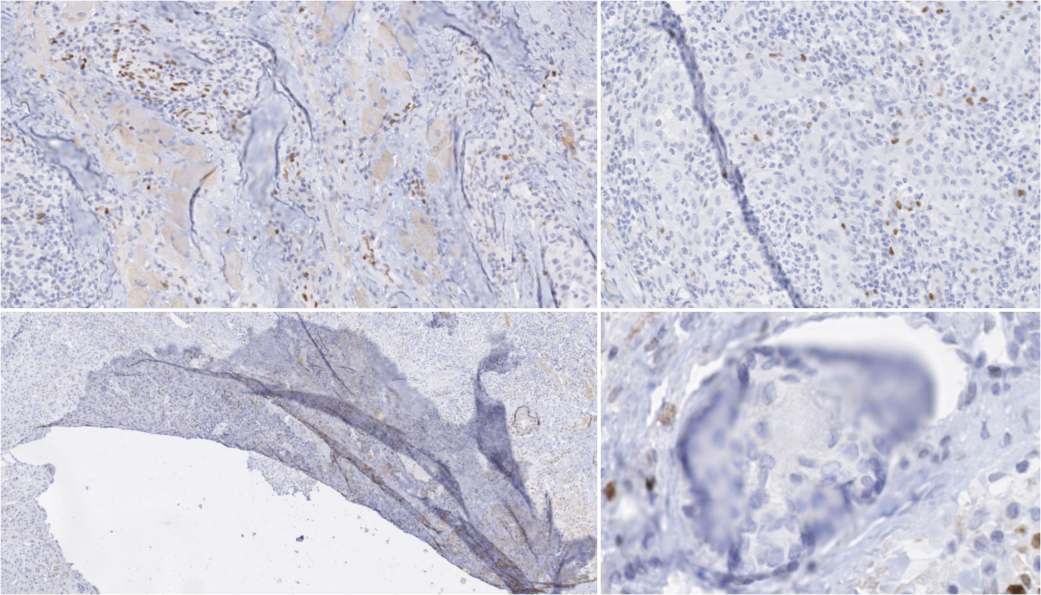
Rolls and Farmer define an artefact in histology or cytology as “a structure that is not normally present in the living tissue” [15]. Artefacts can be by-products of every step of the histopathology tissue processing workflow. Kanwal et al. [12] list and show examples of some common types of artefacts at various stages of the WSI acquisition pipeline:
Damage of the tissue, which can happen during the biopsy or resection, during paraffin block sectioning (e.g. tears, shown in the bottom-left of Figure 6.1), or during staining.
Artefacts on the slide during coverslipping, such as dirt, air bubbles or pen markings on the glass coverslip.
Scanning artefacts, with the most common being blur and stitching artefacts (as scanners often acquire “tiles” which are then stitched together to form the WSI).
While some artefacts are easily distinguished by pathologists, the distinction between “artefact” and “normal tissue” may sometimes be difficult to make [16]. In automated image analysis of histological slides, artefacts can cause potential mistakes in quantitative analyses. Automated segmentation of artefacts may therefore improve the results of such quantitative processing by excluding artefactual tissue. It also provides a mean of controlling the quality of the workflow of a laboratory, to assess the usability of a WSI for diagnostic purpose or to signal if a re-cut, re-staining or re-scanning of the tissue sample may be necessary [9].
The problem of artefact segmentation also illustrates well the difficulties of digital pathology image analysis covered in this thesis. As the frontier between “artefact” and “normal tissue” is not well-defined, pathologist scoring of the WSI quality has a relatively high interobserver variability [5]. As the boundaries of the artefact are very difficult to strictly define, there will be a large uncertainty on the exact extent of the artefactual region. The diversity in nature, shape and size of the artefacts (see Figure 6.1) also make it extremely difficult for an expert to exhaustively annotate artefactual regions, making the quantitative evaluation of the automatic artefact segmentation results very challenging as well.
In our 2018 publication [7], we tested several deep learning strategies for the segmentation of artefactual regions. We later used our artefact dataset as a case study for some of the “SNOW” experiments [6], and developed a prototype for an automated tool for analysing WSI in a pathology workflow. Several similar tools were in the meantime developed by other research teams, such as Case Western Reserve University’s HistoQC [2], or more recently PathProfiler from the Institute of Biomedical Engineering of the University of Oxford [9].
In this chapter, we will first present the state of the art of artefact detection and segmentation as it stood before our 2018 publication, i.e. before deep learning methods were proposed for this application. We will then present our experiments and results. We will finally explore the latest advances and the current state-of-the-art and discuss how these results may help the pathology practice.
6.1 State of the art before deep learning
Most of the literature on artefact detection focuses either on one or few specific artefacts (most commonly, blur or tissue-folds), or on computing an overall “quality score” for the slide, generally based on blur, noise or contrast [12]. Before our 2018 experiments, all the proposed methods were based on traditional image analysis pipelines with handcrafted features. In this section, we present the state-of-the-art methods for overall quality assessment, blur detection and tissue-fold detection for those traditional methods.
6.1.1 Quality assessment
As the quality assessment of a slide is an important use case for artefact segmentation, many algorithms focus solely on determining an overall objective quality score rather than trying to find specific instances of artefacts. Moreover, these quality scores are often mostly concerned with acquisition artefacts, such as blur or noise. “Sharpness” and “noise,” with sometimes the addition of other general features such as contrast or colour separation, serve as the basis for several quality scores, such as those proposed by Hashimoto et al. [10], Ameisen et al. [1], Shrestha et al. [20] or Shakhawat et al. [19]. The evaluation of such methods is particularly difficult, and generally consists in verifying a correlation with a subjective assessment by a panel of experts. All of these algorithms are relatively straightforward, using gradients, edge detection, and simple neighbourhood operators to determine the relevant statistics, with a linear combination of the individual components providing an overall score.
6.1.2 Blur detection
Blur is the most common acquisition artefact. As the focus parameters of the scanner needs to be adapted during the acquisition depending on the local tissue thickness of the slide, some regions may end up out-of-focus [13]. If quickly detected, it is also a relatively easy artefact to fix, as it only requires the re-acquisition of the out-of-focus regions.
Methods aiming at specifically finding the blurry regions in the whole slide generally take the form of a tile classification algorithm. If the size of the tile is small enough, this provides sufficient precision for the localization of the blurry region, particularly if the aim is to guide re-acquisition rather than to exclude the region from further processing.
Moles Lopez et al. [13] combine the “sharpness” and “noise” features from Hashimoto et al. [10]’s quality score with several other features based on the gradient image and the grey-level cooccurrence matrix statistics. A Decision Tree classifier is then trained on the features to provide a tile classification model.
Similarly, Gao et al. [8] use a diverse set of local features (contrast, gradient, intensity statistics, alongside some wavelet features) and train a set of “weak” Linear Discriminant Analysis classifiers, combined together using AdaBoost. A large set of intensity-based, gradient-based and transform-based features is used by Campanella et al. [4] to train a Random Forest classifier.
These methods show that relatively simple feature-based algorithms obtain good results for blur detection.
6.1.3 Tissue-fold detection
Tissue-folds are very commonly found in pathology tissue, caused by the thin tissue folding on itself while being manipulated. This is particularly common around tears in the tissue, as shown in the bottom-left of Figure 6.1.
One of the earliest tissue-fold detection method was proposed by Palokangas et al. in 2007 [17]. They observed that tissue-fold regions are characterized by a high saturation and low intensity, and used an unsupervised approach with k-means clustering to segment the folds from the rest of the slide. This “high saturation, low intensity” characteristic was also exploited by Bautista et al. [3], who proposed a simple image enhancement function: , where is the enhanced image, the original image, the saturation and the intensity value. A simple luminosity thresholding can then be applied on the enhanced image to segment the tissue folds.
This method is further refined in Kothari et al. [14] in 2013, which also uses to separate the folds from the rest of the tissue but add a method for adapting the threshold to the image being considered. These authors note that, by varying the threshold on the image, the number of connected components is initially low (as most pixels are segmented and therefore merged into a few large regions), then grows rapidly to a peak (as the segmentation includes tissue-folds regions as well as many disjointed nuclei) before going down as only the tissue-fold regions remain. Two thresholds are computed based on the number of connected objects at the peak, and pixels are labelled as “tissue-fold” if their value is larger than the lower threshold and they are in the 5x5px neighborhood of a pixel whose value is larger than the higher threshold.
More recently in 2020, Shakhawat et al. [19] use gray-level cooccurrence matrix statistics and pixel luminance as features to train a SVM on tile-based tissue-fold classification. They also use the same approach for air bubble detection.
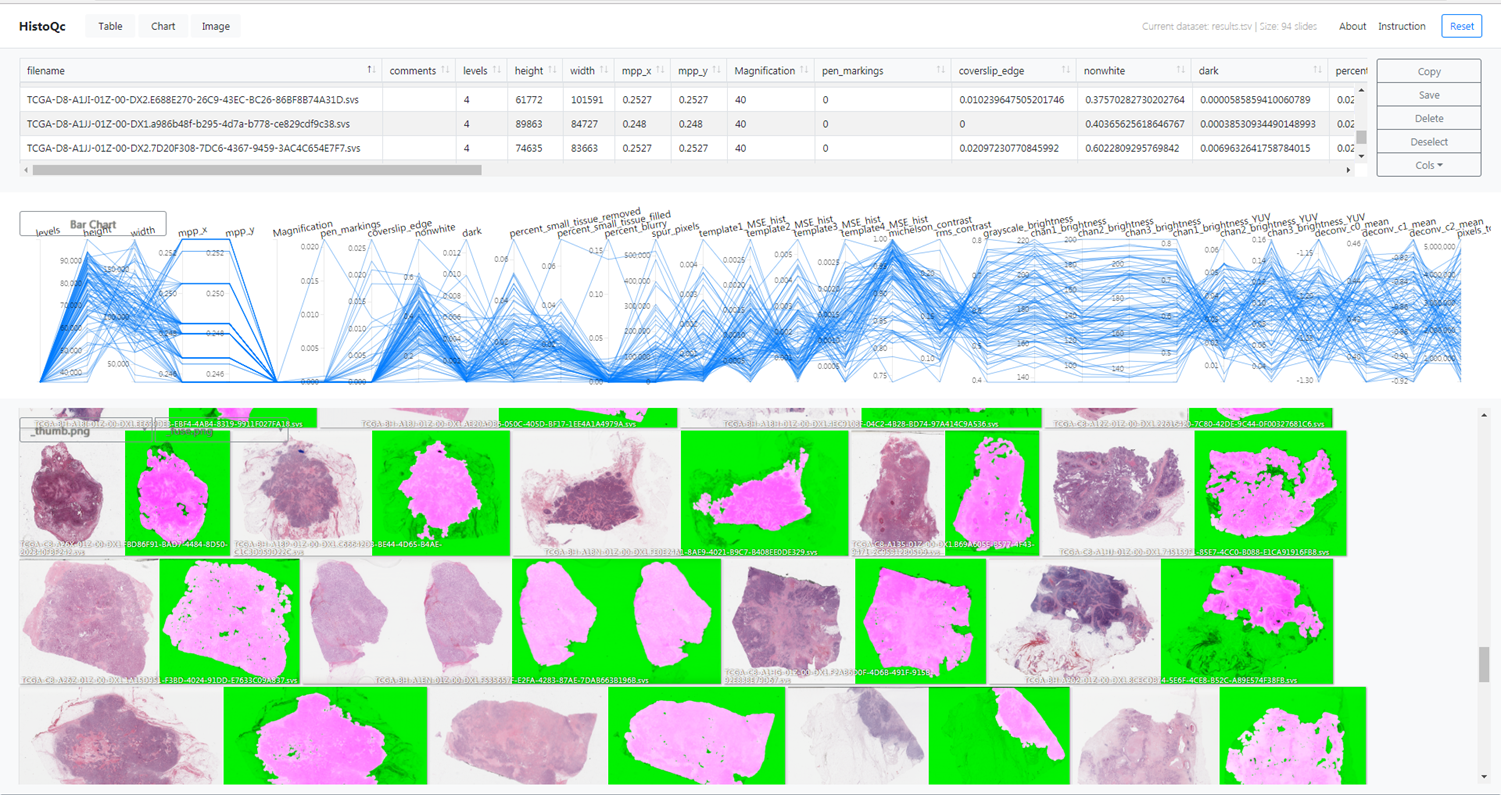
6.1.4 HistoQC
HistoQC is an “open-source quality control tool for digital pathology slides”[^42]. It was initially presented in a 2019 publication by Janowczyk et al. [2], with further experiments and validations presented in a 2020 publication by Chen et al. [5]. It proposes a collection of modules that each target a specific type of artefact. Ad-hoc pipelines can be created in a configuration file to apply those modules to a target WSI. It also provides a web-based interface to visualize the results, shown in Figure 6.2. The result of the pipeline is a set of statistics describing the different aspects of the quality of the slide, and a mask separating the normal tissue from the background glass slide and the artefacts (which include air bubbles, pen markings, tissue-folds, and blurry regions).
The software was validated in the 2019 publication [2] in a qualitative analysis involving two expert pathologists who determined whether the results proposed by the software were “acceptable” (defined as “an 85% area overlap between the pathologists’ visual assessment and the computational assessment by HistoQC of artefact-free tissue”) on a set of 450 slides. They reported an agreement on 94% and 97% of the slide with the two experts (similar to the 96% inter-expert agreement). In the larger 2020 experiment involving three pathologists and 1800 slides [5] (but limited to renal biopsies), they showed the potential of this type of software as an aid to the pathologist, reporting a considerable improvement in inter-expert agreement when using the software than when assessing the quality of the slide without the help of the application.
6.2 Experimental results
Our first experiments on artefact segmentation were presented at the CloudTech conference in 2018 [7], but our main work on the topic was included as a case study in our SNOW experiments in 2020 [6]. We will focus here on the latter results, which we report and extend.
6.2.1 Materials
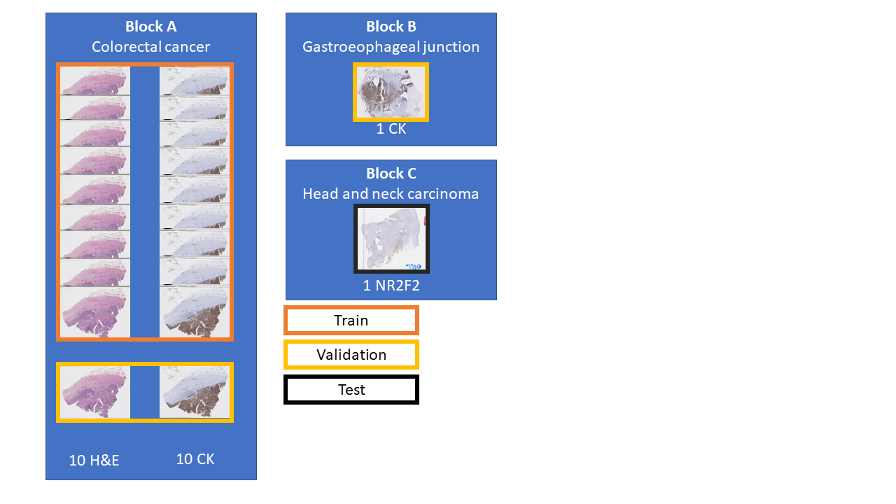
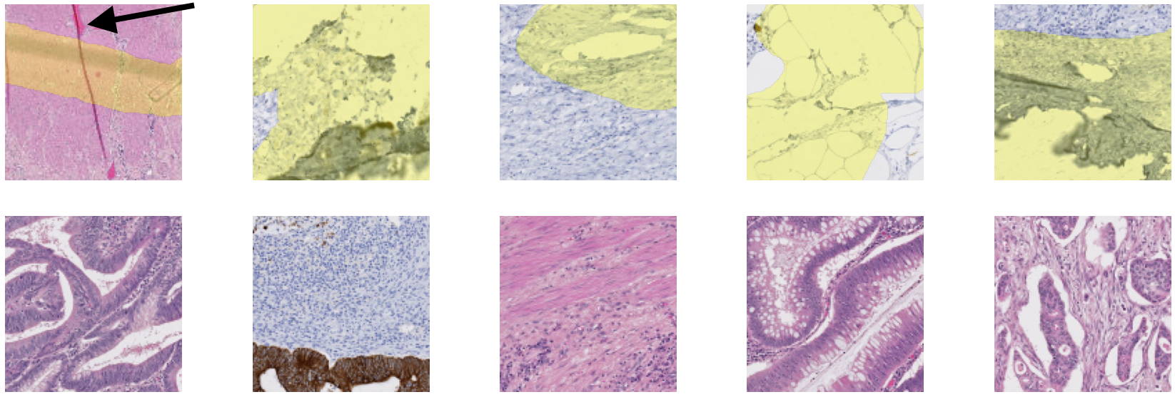
A full description of our artefact dataset can be found in Annex A, and a visual summary is shown in Figure 6.3. The dataset contains WSIs extracted from three tissue blocks. Twenty slides come from a colorectal cancer tissue block (“Block A,” 10 with H&E staining, and 10 with anti-pan-cytokeratin IHC staining). One from a gastroesophageal junction tissue block (“Block B,” stained with anti-pan-cytokeratin IHC), and one from head and neck carcinoma (“Block C,” with anti-NR2F2 IHC staining). The annotations for the training set (18 slides from Block A) and the validation set (2 slides from block A and one from block B) were done by the author. They are weak (with approximative contours) and noisy (few of the annotated objects should be incorrect, but many small artefacts are not annotated). The test slide (from block C) is annotated by a histology technologist. However, while the quality of the annotations is much better than in the training and evaluation set, there are still many missing small artefacts, and the exact boundaries are still uncertain. An important characteristic of the dataset (especially compared with the challenge datasets used in Chapter 5) is the scarcity of the “positive” class (in this case, artefactual regions). In the training set, only 2% of the pixels are annotated as “positive.” In the validation set and the test slide, where more care was taken to be as exhaustive as possible in the annotations, this ratio increases to 7% and 9%, respectively. Examples of annotated tiles from block A are shown in Figure 6.4.
6.2.2 Methods
As in the previous SNOW experiments, the ShortRes, PAN and U-Net architectures were used. In terms of learning strategies, the baseline, GA50 and Only Positive strategies were chosen based on the results of the experiments on the corrupted GlaS and Epithelium datasets reported in Chapter 5.
An insight from our early experiments was that the very large uncertainty on the annotations made the quantitative assessment of the performance of the algorithms difficult. Typical segmentation or per-pixel classification metrics (such as DSC, SEN, SPE…) generally failed to capture much useful information about the relative strengths and weaknesses of the trained networks. The qualitative evaluation was generally more informative and easier to relate to the potential for practical use of the system in a laboratory setting.
The evaluation method was therefore adapted to have a more qualitative approach. Twenty-one tiles or varying dimensions (between around 400x400 and 800x800px) were extracted from the three “validation” slides (see Figure 6.3). Eight of the 21 test tiles have no or very few artefact pixels. The others show examples of tissue tears & folds (6), ink stains (2), blur (2), or other damage.
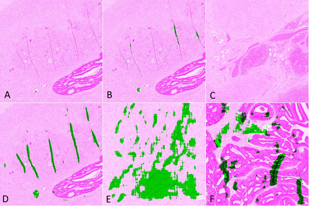
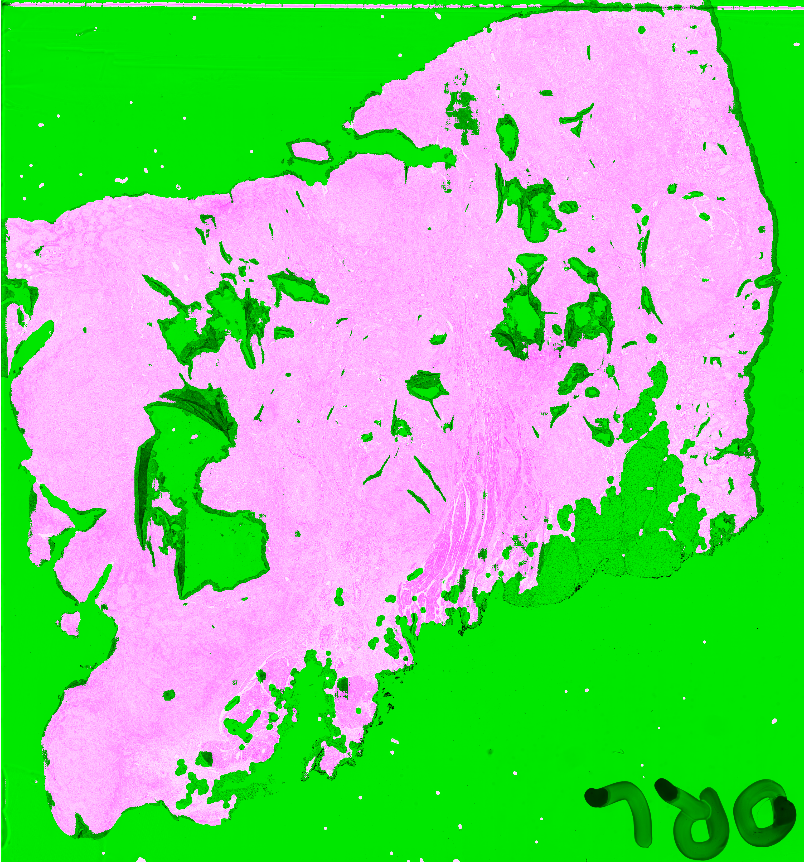
For each slide and network, we classify the result on each test tile as Good (results are acceptable), False Negative (some artefacts are not detected or the segmented region is too small), False Positive (some tissue regions without artefact are segmented), or Bad (completely misses artefacts or detects too much normal tissue as artefacts). Examples of such results are illustrated in Figure 6.5, where tissue regions considered as normal are shown in pink and those considered as artefactual are shown in green, using the visualisation convention proposed in HistoQC [2].
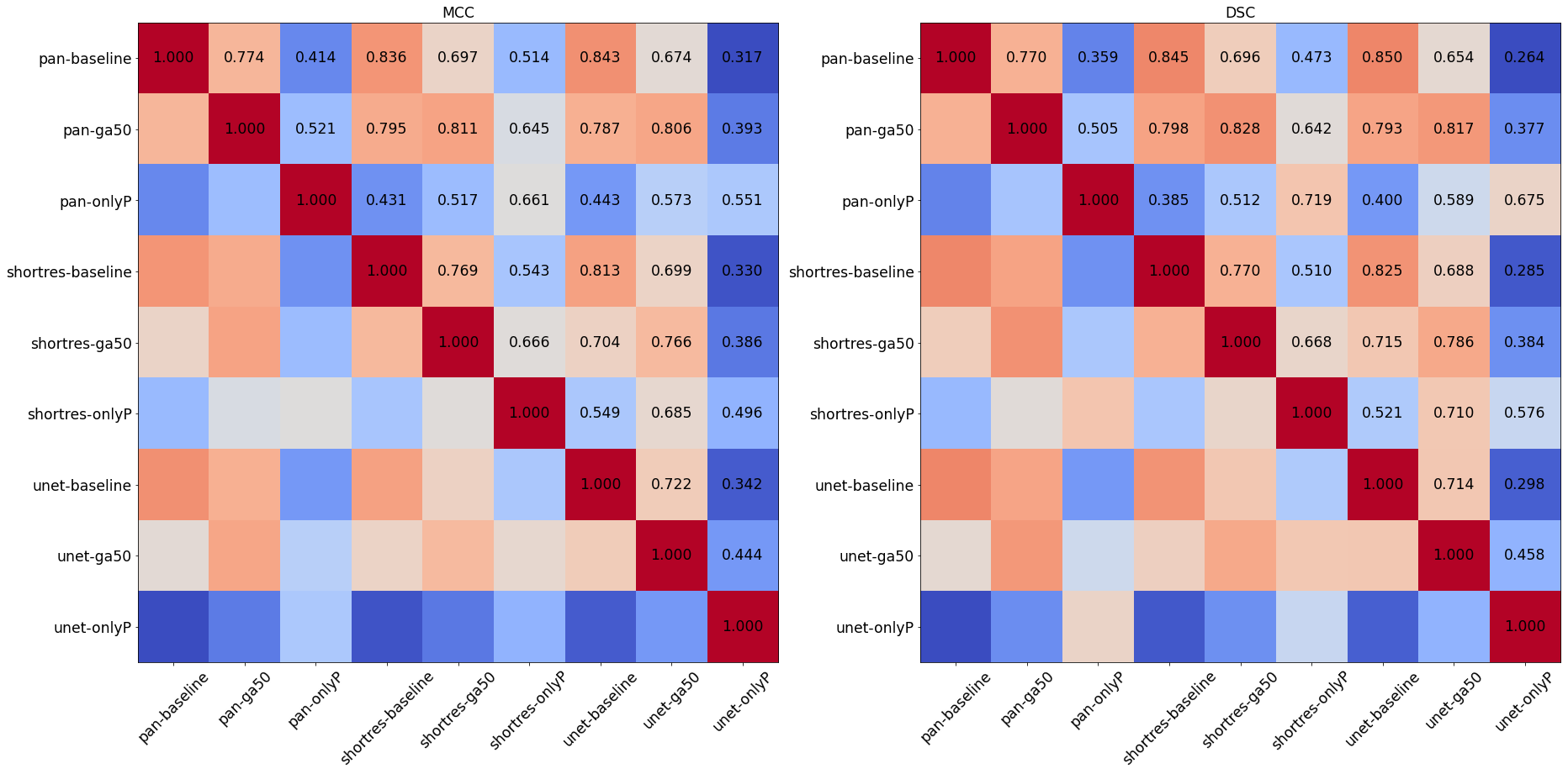
To compare the results of the different strategies and networks, we score the predictions on each tile by giving penalties according to the type of error (Good = 0, False Positive = 1, False Negative = 2, Bad = 3). False positives are given a lower penalty than false negative, as it is typically better to overestimate an artefactual region than to misidentify an artefact as normal tissue. We compute the sum of the penalties on all 21 tiles to get a final penalty score, a lower penalty score thus meaning a better strategy. While we have seen that quantitative metrics are poor indicators for the performances of the algorithms in the absence of an objectively and correctly annotated ground truth, they can still be useful as a measure of similarity between the predictions of the different methods (thus comparing the methods with each other rather than with the annotations). We compute the DSC and the per-pixel MCC of each algorithm compared with each other to form similarity matrices, which are used to generate an MDS visualisation of the similarity between algorithms (as already used in section 4.4.5).
The last slide from Block C, which is distinguished from the others by the tissue origin and the IHC marker (see Figure 6.3), is used to visually assess the results on an independent whole slide image. Additionally, four H&E slides from the TCGA database containing different types of artefacts (identified in the "HistoQC Repository[^43]") are added as an external dataset for the qualitative evaluation.
For whole-slide prediction, we first perform background detection (i.e. glass side without tissue) by downscaling the image by a factor of 8, converting the image to the HSV colour space, and finding background with a low saturation (). The resulting background mask is rescaled to the original size and fused with the artefact segmentation result. All slides are analysed at 1.25x magnification. We use a regular 128x128 pixels tiling of the whole slide with 50% overlap and keep the maximum output of the artefact class for every pixel.
6.2.3 Results on the validation tiles
The results on the validation tiles are shown in Table 6.1. The GA50 strategy consistently performs better than the baseline and Only Positive for all three network architectures. The Only Positive strategy consistently overestimate the artefactual region, with the largest FP number, while the baseline network tends to underestimate it. In this case of low density of objects of interest, the results show that limiting the training only to annotated regions and regions close to annotations is too restrictive. It should be also noted that for the three networks the GA50 strategy is able to retrieve all the "bad" cases from the baseline, which seems less accurate with PAN and U-Net than with ShortRes.
| ShortRes | Good | FP | FN | Bad | Penalty Score |
|---|---|---|---|---|---|
| Baseline | 14 | 0 | 5 | 2 | 16 |
| GA50 | 16 | 1 | 4 | 0 | 9 |
| Only Positive | 13 | 7 | 0 | 1 | 10 |
| PAN | Good | FP | FN | Bad | Penalty Score |
| Baseline | 13 | 0 | 5 | 3 | 19 |
| GA50 | 19 | 0 | 2 | 0 | 4 |
| Only Positive | 8 | 12 | 0 | 1 | 15 |
| U-Net | Good | FP | FN | Bad | Penalty Score |
| Baseline | 13 | 0 | 6 | 2 | 18 |
| GA50 | 19 | 1 | 1 | 0 | 3 |
| Only Positive | 3 | 10 | 0 | 8 | 34 |
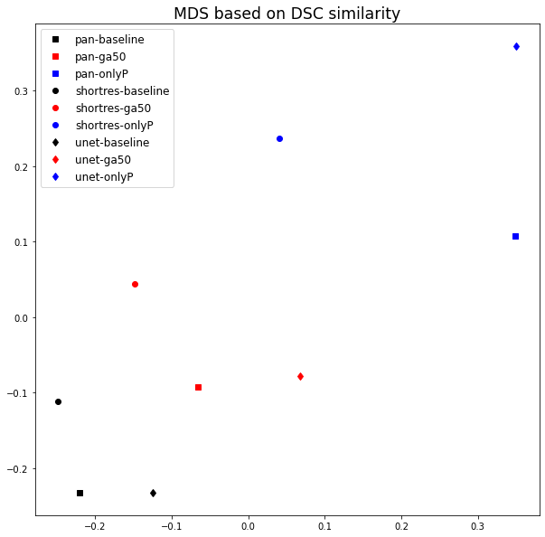
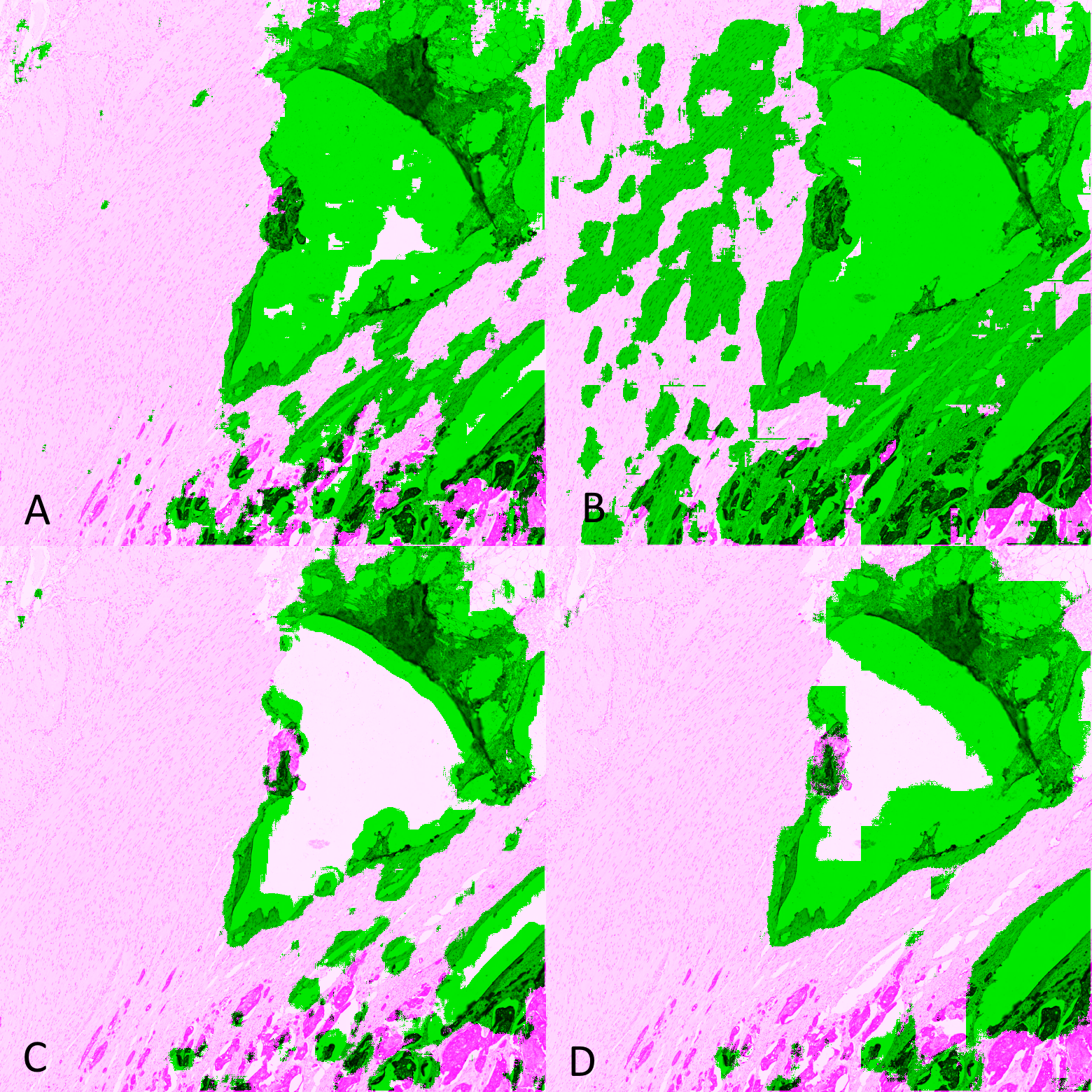
The comparisons between the different algorithms using the DSC and per-pixel MCC are reported in Figure 6.6, and the MDS visualisation of the dissimilarity (using the DSC) is shown in Figure 6.7. It is immediately apparent that the main driver of the similarity between the results of the methods is the learning strategy rather than the network architecture. The Only Positive strategy has a much larger spread to its cluster than the two others, indicating that its results are more network-dependent than the two other strategies. This is illustrated in Figure 6.8, where we can see for one of the validation tiles that the Only Positive strategy predicts a lot more false positive artefacts with the U-Net than with the ShortRes network, while the GA50 has much more similar predictions between the two networks.
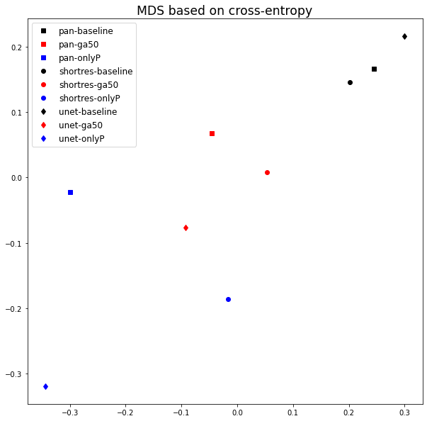
The bad results of the Only Positive method, however, may be in part attributable to the fixed 0.5 threshold used to produce the prediction mask from the pixel probabilities. If, instead of the MCC or DSC, we compute the average cross-entropy between the probability maps of the networks and build a similarity matrix, the MDS visualisation (Figure 6.9) shows that the predictions of the PAN and ShortRes Only Positive networks are much more similar to the GA50 networks than was apparent from the binarized predictions. The GA50 appears in both cases to be a “compromise” between the OnlyP and baseline strategies.
6.2.4 Results on the test slides
Given the results on the validation tiles, the PAN-GA50 network was used on five test whole-slide images for a qualitative evaluation: the “Block C” slide (see Figure 6.3) and four slides from the TCGA dataset, chosen for the presence of different types of artefacts as identified on the HistoQC repository. Our observations are summarized in Table 6.2, and all the predictions are shown in Figure 6.10-Figure 6.14. It should be noted that the processing time for PAN-GA50 took around 2 minutes 20 seconds for the 4 TCGA slides using an NVIDIA TITAN X GPU.
| Slide | (Main) artefacts | PAN-GA50 result |
|---|---|---|
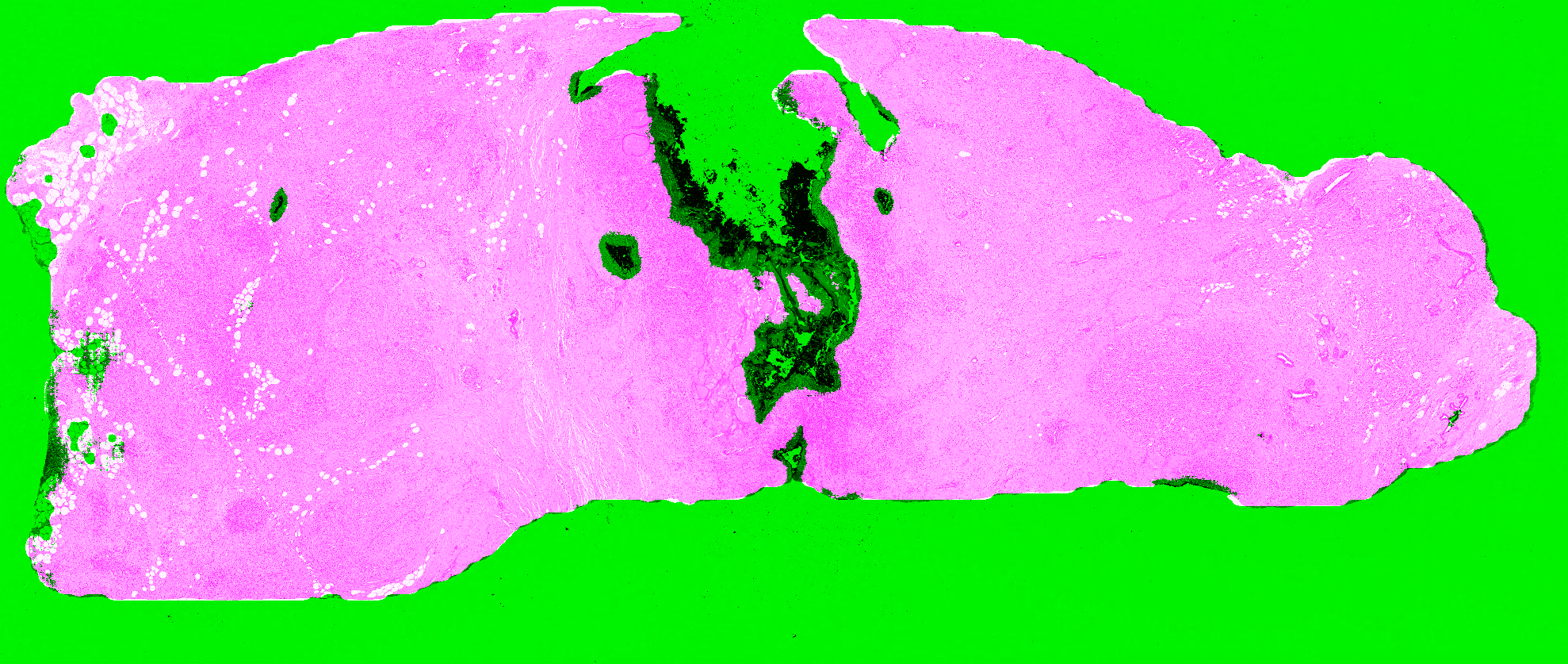
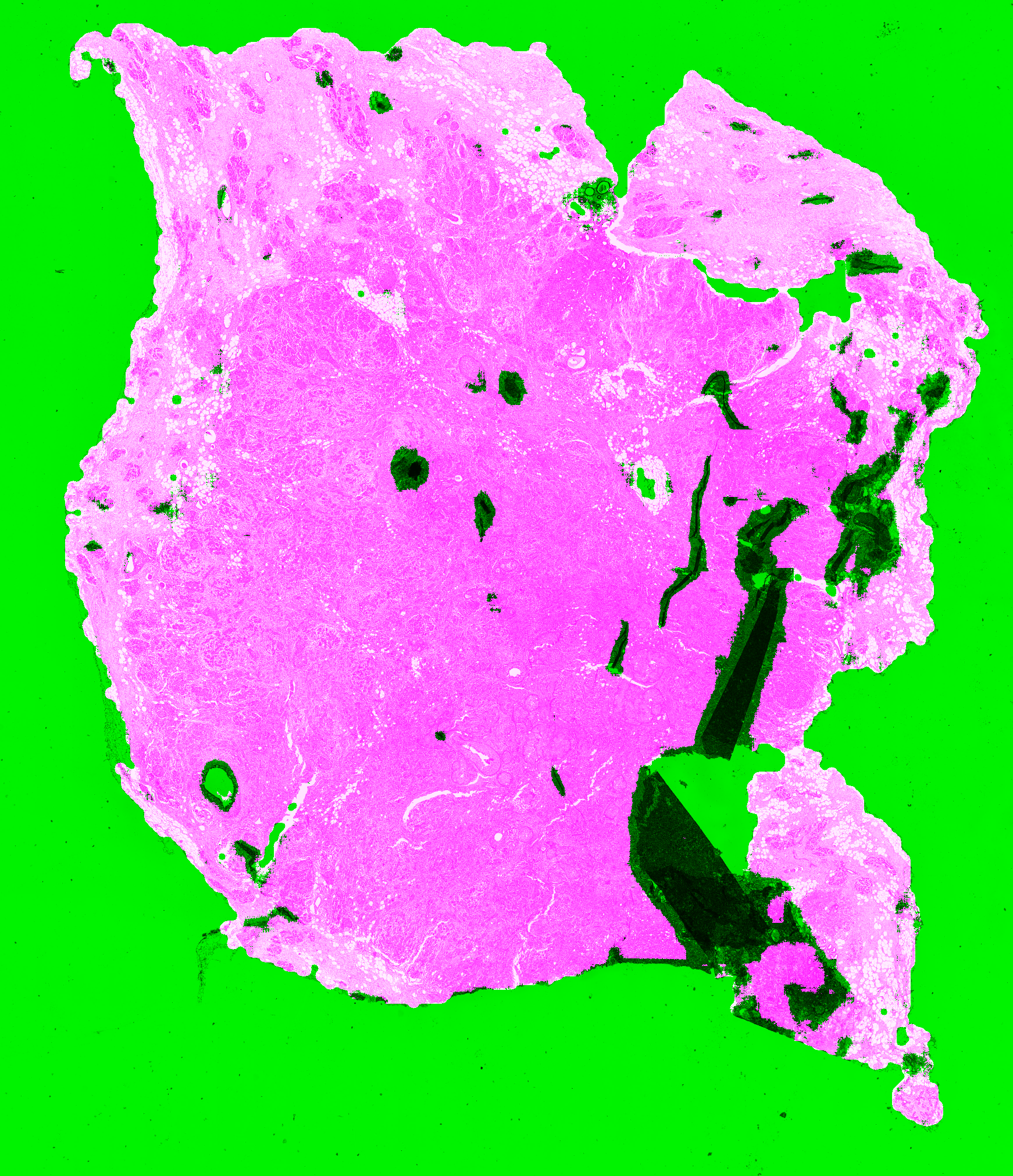
| Block C | Tears and folds | PAN-GA50 misses some small artefacts but its results are generally acceptable. (Figure 6.10) |
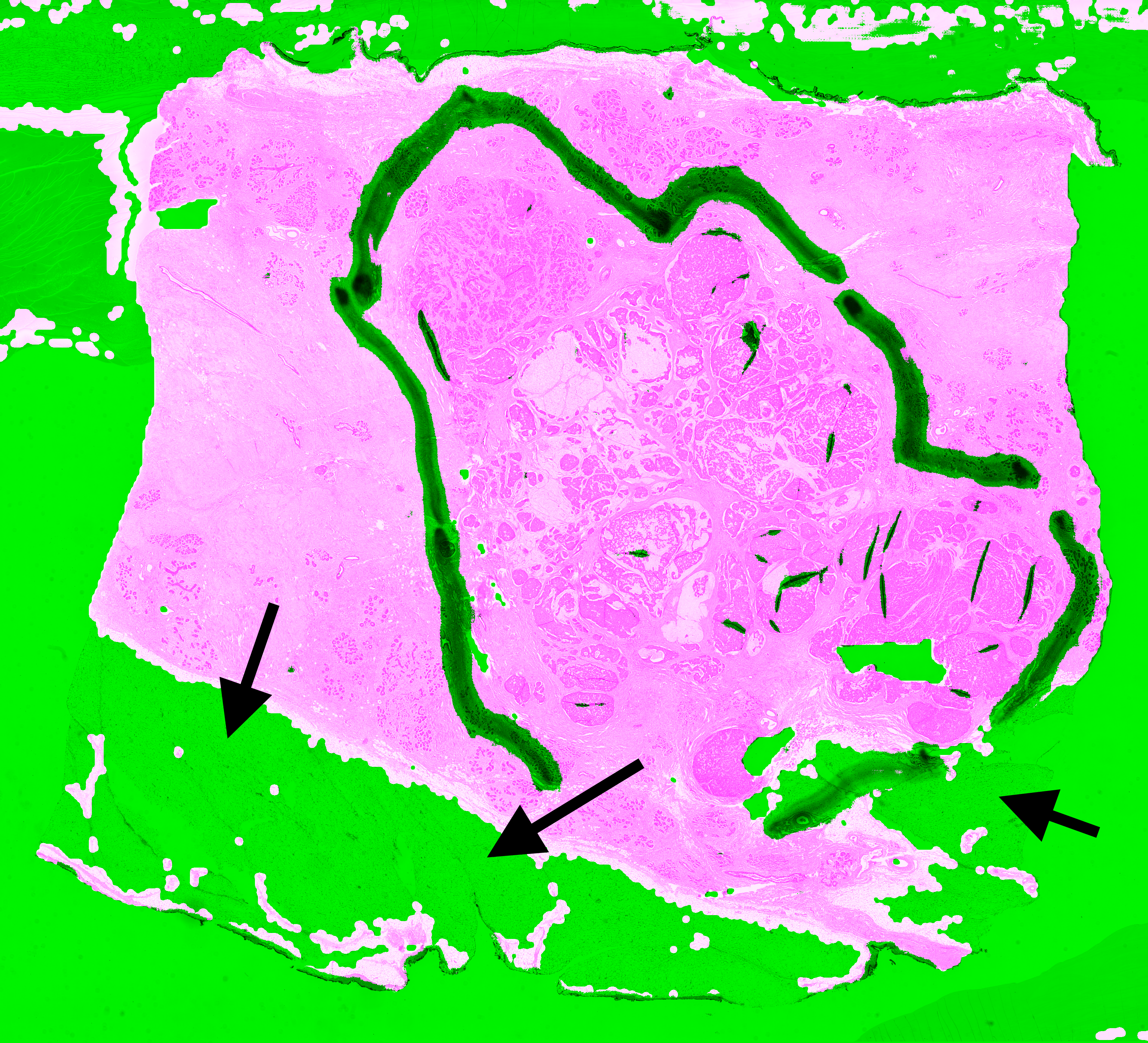
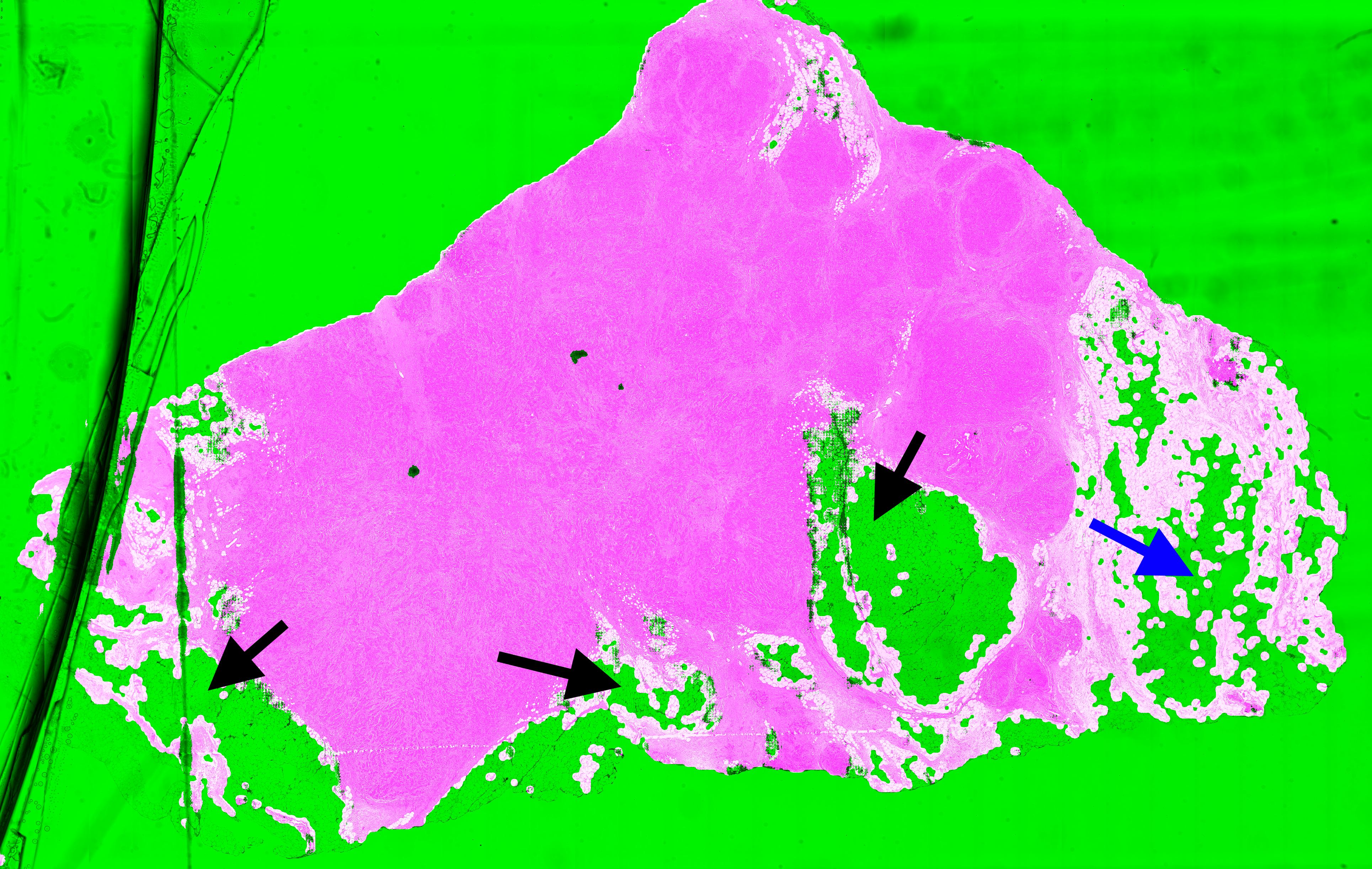
| A1-A0SQ | Pen marking | Pen marking is correctly segmented and small artefacts are found. Some intact fatty tissue is mistakenly labelled (see black arrows in Figure 6.11). |
| AC-A2FB | Tissue shearing, black dye | The main artefacts are correctly identified. (Figure 6.12) |
| AO-A0JE | Crack in slide, dirt | Some intact fatty tissue is mistakenly labelled (see black arrows in Figure 6.13), but all artefacts are found and almost all intact tissue is kept. |
| D8-A141 | Folded tissue | The main artefacts are correctly identified. (Figure 6.14) |
The most recurrent error in the test slide predictions is found in fatty tissue. This tissue has a very distinct appearance (looking like large, empty cells), and were not present in the training dataset. They are therefore likely confused with small holes, and thus identified as artefactual regions.
6.2.5 Insights from the SNOW experiments
Our GA method succeeds in learning from a relatively small set of imprecise annotations, using images from a single tissue type. It generalizes well to new tissue types and previously unseen IHC markers. This method provides a good compromise between using as much of the available data as possible (as in semi-supervised methods) and giving greater weight to the regions where we are more confident in the quality of the annotations (as in the Only Positive strategy). The baseline method underestimates the artefactual region, as expected from the low density of annotated objects in the dataset. The Only Positive strategy, on the other hand, is too limited in the data that it uses and, therefore, has too few examples of normal tissue to correctly identify the artefacts.
While the PAN network was slightly better than the ShortRes network with the GA50 strategy on the test tiles, it performed worse with the Baseline version. Since ShortRes is significantly simpler (20x less parameters), these observations suggest that for problems such as artefact detection, better learning strategies do not necessarily involve larger or more complex networks.
By using strategies adapted to SNOW annotations, we were able to obtain very good results on artefact segmentation with minimal supervision. Extending the network to new types of artefacts or particular appearances of the tissue (such as fat) should only require the addition of some examples with quick and imprecise annotations for fine-tuning.
6.3 Prototype for a quality control application
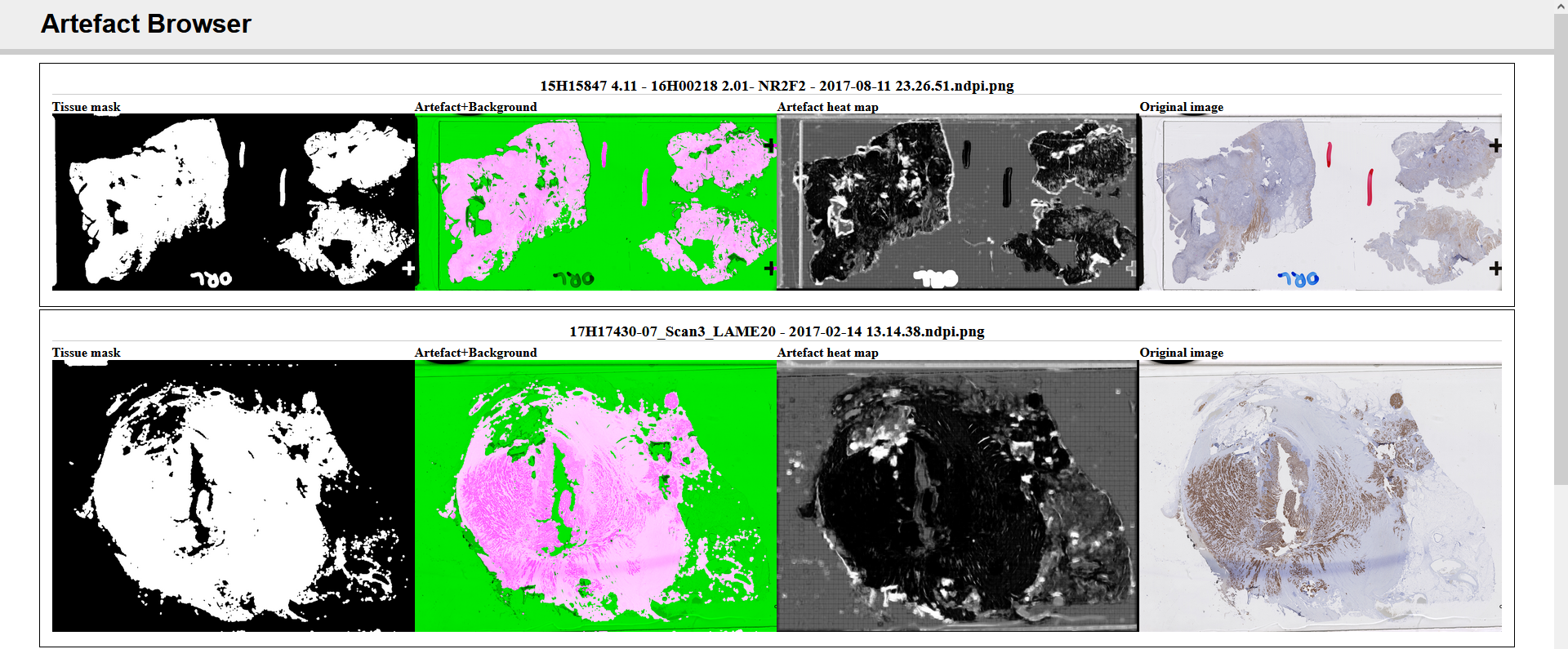
To study the possibility of including our network trained for artefact segmentation in a laboratory environment for quality control, a prototype application was developed with a web-based interface for quickly visualising the quality of newly acquired WSIs. A diagram showing the general concept of the application is shown in Figure 6.15, and a screenshot of the web interface in Figure 6.16. The overall architecture of the application is largely based on HistoQC, except that it uses our trained PAN-GA50 network to segment all artefacts instead of their classic image analysis approach, and it requires no specific configuration for each WSI, as our model generalizes well to different stains and organs.
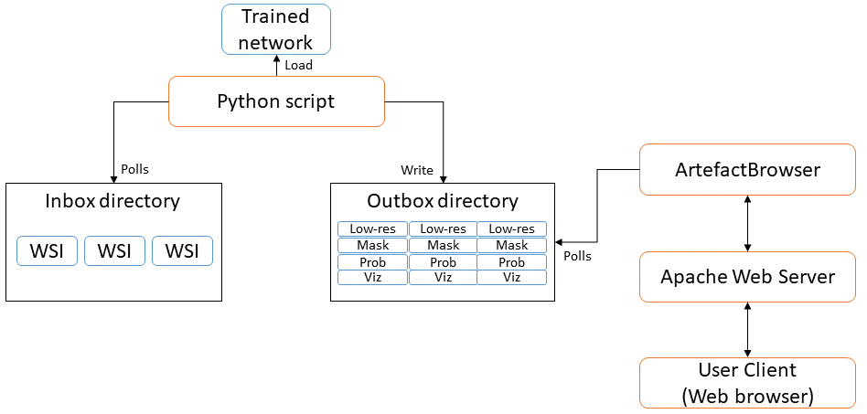
Such a system could be introduced into a pathology laboratory workflow to provide quick feedback on the quality of the acquisitions. Quantitative measurements can additionally be made based on, for instance, the ratio of artefactual tissue to normal tissue (excluding the background glass slide). Development and validation of the prototype was however postponed as the coronavirus crisis necessarily shifted the priorities of the pathology laboratory involved in the process.
6.4 Recent advances in artefact segmentation
Several recent software and publications have addressed the problem of artefact segmentation more recently. The PathProfiler open-source software[^44] by Haghighat et al. [9] uses a U-Net network to separate tissue from the glass slide background, and a multi-label regression network with a ResNet-18 backbone to predict the quality of 256x256px patches extracted at 5x magnification. The scores predicted per patch are a general “usability” score, the probability of “no artefact” in the patch, and the quality of the patch with regards to staining issues, focus issues, folding artefacts and “other artefacts.” Performances are evaluated based on the Pearson correlation coefficient between the algorithm and the expert on the overall usability score, and patch-level ROC-AUC based on expert annotations.
Deep learning methods have also been proposed more specifically for the detection of blurry regions, like Senaras et al.’s DeepFocus [18] which uses a very straightforward classification architecture similar to AlexNet. Swiderska-Chadaj et al. [21], meanwhile, train a U-Net network on “damaged tissue, which include”distortions, deformations, folds and tissue breaks" in Ki-67-stained brain tumour specimens. Their qualitative results seem good, but their evaluation is based only on annotated patches and do not include WSI predictions, making it harder to fully assess the quality of their final product.
The effect of artefacts on deep learning algorithms for digital pathology image analysis was analyzed by Schömig-Markiefka et al. [11]. They used different types of artificially generated artefacts (focus, compression, contrast, deformation, bad staining, dark spots…) and observed the decrease in performance of a tumour patch classification algorithm. They notably found that “substantial losses of accuracy can occur when the focus quality levels are still visually perceptible as adequate by pathologists,” and that “any [JPEG] compression levels under 80% can result in accuracy deterioration.” In general, they demonstrate that all artefacts “might result in accuracy deterioration and warrant quality control measures.”
6.5 Discussion
From our experiments and the state-of-the-art, it seems relatively clear that the difficulty in artefact detection and segmentation is found not so much in the ability of deep neural networks to find relevant and accurate features, but rather in the very loose definition of the problem itself. This leads to a scarcity of good expert annotations, and to the impracticality of quantitative evaluations. Most of the proposed evaluation methodologies (including ours) rely on subjective assessment by experts of the “quality” of the slide, or of the predicted artefactual region.
These results, however, tend to show that automated segmentation of artefactual regions, either as a pre-processing step before running other image analysis tasks or as a quality control step just after the acquisition of the slide, is a good use case for deep learning methods. Our experiments show that even a limited supply of low-quality annotations (with all WSIs from the training set coming from the same block) results in a trained network with good generalization capabilities (to other organs and staining agents).
Tools such as HistoQC, PathProfiler, or our prototype application can easily be integrated into a digital pathology workflow, providing a quick automated analysis of the quality of the WSI to warn against the necessity of re-staining or re-acquiring a slide, and to provide objective quality control metrics for a laboratory’s assessment of the quality of their output.
The performance of HistoQC shows that even relatively simple methods can give good results for this application. The main drawback of that system, however, is the necessity to tweak the configuration depending on the nature of the slide to analyse. The deep learning methods such as PathProfiler’s or ours, meanwhile, are easier to use out-of-the-box on new examples but require some time investment to annotate examples of the type of artefactual regions that are relevant to detect for the purposes of the laboratory. As the annotations do not have to be very precise, however, this time investment is more limited than in most “clinical” applications and can more easily be outsourced to non-experts based on a smaller set of expert examples.