---- 3.1 Mitosis detection in breast cancer
------ 3.1.1 MITOS12 and MITOS-ATYPIA-14 ICPR challenges
------ 3.1.2 AMIDA13 & TUPAC16
------ 3.1.3 MIDOG 2021
---- 3.2 Tumour classification and scoring
------ 3.2.1 Generic classification
------ 3.2.2 Scoring systems
---- 3.3 Detection, segmentation, and classification of small structures
---- 3.4 Segmentation and classification of regions
---- 3.5 Public datasets for image analysis in digital pathology
---- 3.6 Summary of the state-of-the-art
------ 3.6.1 Pre-processing
------ 3.6.2 Data augmentation
------ 3.6.3 Network architectures
------ 3.6.4 Pre-training and training
------ 3.6.5 Post-processing and task adaptation
---- 3.7 The deep learning pipeline in digital pathology
3. Deep learning in digital pathology
Finding the “first” application of deep learning in digital pathology is difficult, as the definitions are fuzzy. The earliest example that we could find that would qualify as such comes from Malon et al. in 2008 [50]. Using a network architecture based on LeNet-5 (LeCun et al.’s 1998 version of their architecture [43], which is very similar as well to Krizhevsky et al.’s 2012 ImageNet-winning network [39]), they showed that convolutional neural networks were capable of encouraging results on epithelial layer, mitosis and signet ring cell detection.
It is in 2012, however, that deep learning really took off, in digital pathology and in general, with the ICPR mitosis detection challenge (“MITOS12”), won by the IDSIA team of Cireşan et al. with a convolutional neural network [18]. Around the same time, Malon et al. [51] also used a convolutional network for mitosis detection, while Cruz-Roa et al. used a deep learning architecture for basal-cell carcinoma cancer detection [20].
The history of deep learning in digital pathology is strongly linked to the history of “grand challenges.” The first digital pathology competition was organized in 2010 at ICPR (“Pattern Recognition in Histopathological Images”) [30]. It proposed two tasks: counting lymphocytes and counting centroblasts. Five groups submitted their results, none of which used deep learning methods. All subsequent digital pathology challenges, starting with MITOS12, would be won by deep learning algorithms. The ICPR 2010 challenge was mostly an experiment laying the groundwork for future challenges. To quote the authors:
“Given that digital pathology is a nascent field and that application of pattern recognition and image analysis methods to digitized histopathology is even more recent, there is not yet consensus on what level of performance would be acceptable in the clinic.”
The main purpose of the contest was, therefore, “to encourage pattern recognition and computer vision researchers in getting involved in the rapidly emerging area of histopathology image analysis.” The number of challenges grew steadily over the next years, often linked with large conferences such as ICPR, MICCAI and ISBI [32]. As these challenges often published at least their training datasets and annotations, they have been an important source of data for researchers in the domain, either through participation in the challenge themselves, or through further use of the data in later years.
In 2017, when Litjens et al. published their survey on deep learning in medical image analysis [46], they listed 64 publications between 2013 and 2017 on various tasks, including nucleus detection, segmentation and classification; large organ segmentation; and disease detection and classification. They also note how challenges demonstrated the superiority of deep learning methods over “classical” methods, citing the performance of Cireşan et al. [18] in the MITOS12 & AMIDA13 challenges (mitosis detection), alongside the winners of other challenges such as GlaS (gland segmentation), CAMELYON16 (cancer metastasis detection in lymph nodes) and TUPAC16 (tumour proliferation assessment).
The 2018 study by Maier-Hein et al [49] provides a critical analysis of biomedical challenges and their rankings. It demonstrated the lack of robustness of challenge rankings with regard to small variations in the metrics used, in the results aggregation methodology, in the selection of experts for the annotations and in the selection of the teams that are ranked.
In 2020, Hartman et al. published a review of digital pathology challenges [32] listing 24 challenges between 2010 and 2020. Their review focuses on the characteristics of the dataset and the practical value that the challenges have for the pathology community. They note in their conclusion that there is “a disconnect between the types of organs studied and the large volume specimens typically encountered in routine clinical practice” and that this mismatch may “limit the wider adoption of AI by the pathology community.” They also emphasize their value through the fact that “a common evaluation method and dataset allow for a better comparison of the performance of the algorithms,” and that “public challenges also foster the development of AI by reducing the start‑up costs to commence with AI development.”
In our own 2022 review [23], we focus on segmentation challenges and on how they create consensus ground truths from multiple experts, how the evaluation metrics, and the transparency (or lack thereof) that challenges offer with regard to their evaluation code, their datasets and the detailed results of the algorithms.
In this section of the thesis, we will review the use of deep learning in digital pathology, mostly through the lens of challenges. We will first look at the different tasks that challenges have proposed to solve (see Table 3.1), and at how they relate to the generic computer vision tasks that we previously defined. We will then look at how the classic deep learning pipeline adapts to the specificities of digital pathology tasks and datasets.
The main source for finding those challenges is the “grand-challenge.org” website. Some additional challenges were found from being mentioned in other challenge publications, in Maier-Hein’s study [49], or in “The Cancer Imaging Archive” (TCIA) wiki.1 The inclusion criteria for this list are that the dataset is composed of histological images (WSI, Tissue Microarray or patches extracted from either), with either H&E or IHC staining.
| Name, Year | Post-challenge publication or website | Task(s) |
|---|---|---|
| PR in HIMA, 2010 | Gurcan, 2010 [29] | Lymphocyte segmentation, centroblast detection. |
| MITOS, 2012 | Roux, 2013 [60] | Mitosis detection. |
| AMIDA, 2013 | Veta, 2015 [71] | Mitosis detection. |
| MITOS-ATYPIA, 2014 | Challenge website | Mitosis detection, nuclear atypia scoring. |
| Brain Tumour DP Challenge, 2014 | Challenge website | Necrosis region segmentation, gliobastoma multiforme / low grade glioma classification. |
| Segmentation of Nuclei in DP Images (SNI), 2015 | Description in TCIA wiki | Nuclei segmentation. |
| BIOIMAGING, 2015 | Challenge website | Tumour classification. |
| GlaS, 2015 | Sirinukunwattana, 2017 [61] | Gland segmentation. |
| TUPAC, 2016 | Veta, 2019 [70] | Mitotic scoring, PAM50 scoring, mitosis detection. |
| CAMELYON, 2016 | Ehteshami Bejnordi, 2017 [22] | Metastases detection. |
| SNI, 2016 | Challenge website | Nuclei segmentation. |
| HER2, 2016 | Qaiser, 2018 [55] | HER2 scoring. |
| Tissue Microarray Analysis in Thyroid Cancer Diagnosis, 2017 | Wang, 2018 [73] | Prediction of BRAF gene mutation (classification), TNM stage (scoring), extension status (scoring), tumour size (regression), metastasis status (scoring). |
| CAMELYON, 2017 | Bandi, 2019 [10] | Tumour scoring (pN-stage) in lymph nodes. |
| SNI, 2017 | Vu, 2019 [72] | Nuclei segmentation. |
| SNI, 2018 | Kurc, 2020 [41] | Nuclei segmentation. |
| ICIAR BACH, 2018 | Aresta, 2019 [8] | Tumour type patch classification, tumour type region segmentation. |
| MoNuSeg, 2018 | Kumar, 2020 [40] | Nuclei segmentation. |
| C-NMC, 2019 | Gupta, 2019 [28] | Normal/Malignant cell classification. |
| BreastPathQ, 2019 | Petrick, 2021 [54] | Tumour cellularity assessment (regression). |
| PatchCamelyon, 2019 | Challenge website | Metastasis patch classification. |
| ACDC@LungHP, 2019 | Li, 2019 [44] | Lung carcinoma segmentation. |
| LYON, 2019 | Swiderska-Chadaj, 2019 [62] | Lymphocyte detection. |
| PAIP, 2019 | Kim, 2021 [38] | Tumour segmentation, viable tumour ratio estimation (regression). |
| Gleason, 2019 | Challenge website | Tumour scoring, Gleason pattern region segmentation. |
| DigestPath, 2019 | Zhu, 2021 [80] | Signet ring cell detection, lesion segmentation, benign/malign tissue classification. |
| LYSTO, 2019 | Challenge website | Lymphocyte assessment. |
| BCSS, 2019 | Amgad, 2019 [4] | Breast cancer regions semantic segmentation. |
| ANHIR, 2019 | Borovec, 2020 [11] | WSI registration. |
| HeroHE, 2020 | Conde-Sousa, 2021 [19] | HER2 scoring. |
| MoNuSAC, 2020 | Verma, 2021 [68] | Nuclei detection, segmentation, and classification. |
| PANDA, 2020 | Bulten, 2022 [12] | Prostate cancer Gleason scoring. |
| PAIP, 2020 | Challenge website | Colorectal cancer MSI scoring and whole tumour area segmentation. |
| Seg-PC, 2021 | Challenge website | Multiple myeloma plasma cells segmentation. |
| PAIP, 2021 | Challenge website | Perineural invasion detection and segmentation. |
| NuCLS, 2021 | Amgad, 2021 [3] | Nuclei detection, segmentation and classification. |
| WSSS4LUAD, 2021 | Challenge website | Tissue semantic segmentation from weak, image-level annotations. |
| MIDOG, 2021 | Aubreville, 2022 [9] | Mitosis detection. |
3.1 Mitosis detection in breast cancer
In 2008, Malon et al. propose what may be the first “deep learning” algorithm in digital pathology [50], with a CNN “loosely patterned” on the LeNet-5 architecture [43]. For mitosis detection, their algorithms still used a “traditional” technique to detect candidate nuclei, and then used the CNN to discriminate between the mitotic and non-mitotic classes. To manage the very large class imbalance, they oversample mitotic examples so that they constitute 20% of the training set. The network alternates between subsampling layers and 5x5 convolutional layers, and they use simple data augmentation based on rotations by 90° increments and symmetrical reflection. They used a slightly updated version of this method [51] in the MITOS12 challenge, which would really start the deep learning era for mitosis detection and for digital pathology.
3.1.1 MITOS12 and MITOS-ATYPIA-14 ICPR challenges
The 2012 Mitosis Detection in Breast Cancer Histological Images (MITOS12) challenge was the second digital pathology image analysis competition, after the “PR in HIMA” from 2010. Organised by the IPAL Lab from Grenoble with the Université Pierre et Marie Curie and the Pitié-Salpêtrière Hospital in Paris, it is notable as the first to be won by a deep learning method. The IDSIA team of Cireşan et al. won by a comfortable margin from a total of 17 submissions [60]. The challenge used H&E stained 2048x2048px image patches from 50 “High Power Fields,” high resolutions area extracted from 5 WSIs. Each WSI was scanned using three different scanners, evaluated separately, with most participants focusing on the “Aperio” scanner images.
Most participants used a classic pipeline much like those discussed in the previous chapter, with an initial candidate selection using thresholding and morphological operations, followed by feature extraction and candidate classification. The best result among those came from the IPAL team of Humayun Irshad [59], which obtained a F1 score of 0.72 on the Aperio set.
Cireşan et al.’s winning method largely surpassed their result with a F1 score of 0.78 on the Aperio images. They used three DCNNs with a (now) classic “classification” architecture, with a sequence of convolutional and max-pooling layers followed by several dense layers applied to 101x101 image patches. The first DCNN was trained on an artificially “balanced” dataset by taking every mitosis example and an equivalent, randomly sampled amount of non-mitosis example (“mitosis example” meaning any 101x101px patch whose central pixel was closer than 10 pixels from an annotated mitosis centroid). This DCNN will have a very large number of False Positives, but it will tend to have a larger probability of mitosis on samples which look similar to mitosis: other nuclei. The output of this DCNN is therefore used to resample the dataset, this time taking all mitosis example and a much larger number (about 14x as many) non-mitosis examples preferably sampled with a weighting factor based on the output of the first DCNN.
Simple data augmentation (rotations and mirroring) is then used and two DCNNs are trained (with the same macro-architecture, but one slightly smaller than the other), and the final prediction on a patch is given by averaging the results of both on 8 variations of the patch (4 rotations with and without mirroring). The predicted result is used to create a “probability map” on a whole 2048x2048 image with a sliding window method. A post-processing step is then used to clean-up the noisy probability map and find local maxima, which are the final “detection” of the algorithm.
This pipeline is slightly different from the classic method, yet some similarities remain. While the final trained DCNNs used for prediction do not have a “candidate selection” step and directly process the entire image, this “candidate selection” idea can still be found in the training step. The results of the ensemble of two DCNNs are also not used directly, as they produce a very large number of false positives: a post-processing step is necessary to obtain a reasonable detection.
The challenge itself, however, suffers from a few important issues that make its results hard to take at face value. First, it uses a very small amount of WSIs, meaning that the generalisation capabilities of any algorithm are hard to measure. Second, it uses only a single expert for the annotations. As we will see in a later chapter, interobserver variability is very high in mitosis detection, so the results based on a single annotator on a small set are going to be very unreliable. Finally, there is a fundamental design flaw in the challenge dataset, in that the split between the training and the test set was done at the “image patch” level and not at the “patient” level, meaning that patches extracted from the same slide are found in both the training and the test set.
This has a very significant impact on the results, as demonstrated by experiments performed by Élisabeth Gruwé during her Master Thesis [27]. Her results show that switching from a cross-validation scheme that mixes the patients to a leave-one-patient-out scheme reduced the score of her method from a 0.68 F1-score to a 0.54 F1-score.
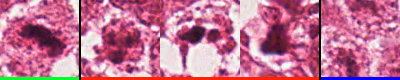
The MITOS-ATYPIA-14 challenge, by the same organisers, addresses those problems by increasing the number of slides to 16, with 5 WSI set aside for testing. It is unclear from the dataset description if some slides came from the same patient. Annotations were independently provided by two pathologists, with a third pathologist’s opinion used to break ties. The supervision files contained information about the potential disagreement by providing a “confidence degree” to each annotated mitosis (see Figure 3.1). No journal publication was made by the 2014 challenge organisers with the results, which are only available on the challenge’s website2.
A post-challenge publication from the winning team of Chen et al. from the Chinese University of Hong Kong [14] explains their method (improved after the challenge), which uses a “cascade” of two patch classification networks. The first “coarse” network is a Fully Convolutional Network, which mostly follows the classic classification macro-architecture, but replaces the “dense” layers by convolutions with a 1x1 kernel, which makes it possible to process an image of an arbitrary size in a single pass. The network is trained with normal dense layers on 94x94px patches, but the dense layers are then converted into 1x1 convolutional layers for the prediction phase so that the network can be applied to the larger image, with each pixel in the output prediction map corresponding to a 94x94px region in the original image. The second, “fine discrimination” model is a patch classification network from Caffe [37], with the weights of the convolutional layers pre-trained on the ImageNet dataset. Three slightly different versions of the model are trained, and their outputs are averaged to provide the final classification.
3.1.2 AMIDA13 & TUPAC16
The AMIDA13 challenge was organised by the UMC Utrecht team of Veta et al. [71]. The dataset contained 2000x2000px image patches extracted from WSIs from 23 patients. Annotations were performed by two pathologists, with two additional pathologists reviewing cases of disagreement. All slides were scanned using an Aperio scanner. As in MITOS12, the IDSIA team of Cireşan et al. was the only “deep learning” approach and won by a clear margin, with an F1-score of 0.61 compared to the next best result of 0.48 by the DTU team of Larsen et al. Cireşan et al.’s method was slightly upgraded from the MITOS12 challenge and used an ensemble of three networks for the prediction, with a post-processing step still necessary.
The TUPAC16 challenge, with the same organising team [70], moved away from just mitosis detection and required the participants to predict the mitotic scores WSIs, in order to make the clinical relevance of the results more important. The mitosis detection performance was also evaluated separately on selected regions from the WSIs. The scoring task used a dataset of more than 800 WSIs, and the mitosis detection task used more than 100 image patches (including the 23 from the AMIDA13 challenge). Both tasks were won by the Lunit Inc.’s team of Paeng et al. [53], which used a ResNet architecture [34] and a two-pass approach where false positives from the first pass are oversampled with data augmentation in the second pass so that the network sees more difficult cases. The panel of competing methods, however, was very different from the previous challenge, as “[w]ith the exception of one team, all participants/teams used deep convolutional neural networks.” The deep neural networks, however, were always included in a larger pipeline, and did not process the WSIs directly: a ROI detection step was almost always included, and for the mitotic score prediction the result of the mitosis detection were often combined with other features in classic machine learning classifiers such as SVMs or Random Forests.
One key insight from looking at the MITOS12, AMIDA13, MITOS-ATYPIA-14 and TUPAC16 results is how important the specificities of the dataset are, even on an identical task, when comparing different methods. Cireşan et al. obtained an F1-score of 0.78 on the MITOS12 set and of 0.61 on the AMIDA13 set with an upgraded method. Chen et al’s post-challenge publication obtained scores of 0.79 on the MITOS12 set, and of 0.48 on the MITOS-ATYPIA-14 set with the same method used in both. The winner of TUPAC16, meanwhile, obtained an F1 score of 0.65 on the mitosis detection score using a ResNet architecture. This makes the evaluation of the potential for clinical applications of these algorithms extremely difficult. As the ground truth for the test sets were not provided for the MITOS-ATYPIA-14, AMIDA13 and TUPAC16 challenges, post-challenge publications are even harder to compare, as even within the same “dataset” the conditions can differ wildly.
As examples, Nateghi et al. [52] showed excellent results using a traditional image analysis pipeline on the 2012 (F1=0.88), 2013 (0.75) and 2014 (0.84) datasets, but they used a five-fold cross-validation scheme and do not specify whether they took the WSI into account in how they created their splits. Similarly, Albaryak et al. [1] have near perfect results (F1=0.97) on the MITOS-ATYPIA-14 dataset with a combination of classic and deep learning methods, but from their description of how they used the dataset, it seems that they worked a balanced subset of the training data, making the problem considerably easier. It is unfortunate that the only dataset where the test data is available is the MITOS12, where the challenge train/test split did not properly take the WSI into account in the first place.
Several deep learning methods have been proposed in recent years, with results that are, as we just saw, difficult to compare. It is still interesting to look at how the methods have evolved since the four challenges.
Cai et al. [13] use the Faster R-CNN architecture [57], a very common object detection network, with a ResNet-101 encoder pre-trained on the ImageNet dataset. Their results illustrate the good performance that can be obtained by retraining general purpose models to the specific tasks of digital pathology. Faster R-CNN was also used by Mahmood et al. [48] in 2020, also with ImageNet pre-training, but this time reverting to a two-pass approach where the Faster R-CNN is used to detect candidate nuclei, and an ensemble of ResNet and DenseNet classification networks is then used to discriminate between the mitosis and non-mitosis nuclei. The pipeline also includes a classic feature extraction & classification step in the middle to refine the candidate list based on handcrafted features. Cai, Mahmood, and a few other methods mentioned in Mahmood et al. used the same train/test split for the MITOS-ATYPIA-14 dataset, making the comparison between them more accurate. Mahmood et al., with a F1 score of 0.69, obtained the best results. It is interesting to note that traditional image analysis methods clearly still play a role in this particular task in state-of-the-art methods, even though off-the-shelf detection networks are starting to perform reasonably well.
3.1.3 MIDOG 2021
The MIDOG challenge was hosted at MICCAI 20213. The dataset contains patches extracted from 280 WSIs acquired with four different scanners. In all the previous challenges there was a lot of variability due to the choice of scanners, and most methods focused on the Aperio datasets, where the results tended to be better. MIDOG chose not to evaluate the different scanners separately, but instead to focus on the “domain generalization” capabilities of the algorithms, pushing participants to create a single model capable of detecting mitosis from any scanner. Two teams obtained essentially equal results: the Tencent AI team of Yang et al. [77] and the TIA Lab team of Jahanifar et al. [35]
Yang et al. use a pre-trained HoVer-Net to detect candidate cells. To help with domain adaptation, they augment the dataset by swapping the low-frequency information in Fourier space of different images, to create new images containing the same high-frequency information (which will contain the object borders) but in the “style” of the images from which the low frequencies (which will contain the overall “background” colour information) were extracted. A SK-UNet [74] segmentation architecture is used to segment the mitotic cells, and a post-processing step cleans-up the segmentation and find the centroid of the object’s bounding boxes as a final detection.
Jahanifar et al. use a stain normalization technique [65] as a pre-processing step, matching the colour space of all images to the same target tile. An Efficient-UNet segmentation model, pretrained on ImageNet, was then used to segment the mitoses. Under-sampling of the negative examples was used during training to provide a balanced dataset to the model. This first network provides a set of segmented candidate nuclei, with many false positives remaining. An Efficient-Net-B7 classification model is then used to further discriminate between mitosis and non-mitosis. An ensemble of three models trained with different subsets of the data during cross-validation is used for inference as the final prediction.
It is clear from this latest challenge that the overall pipeline of mitosis detection remains remarkably similar from one challenge to the next, with the addition of a colour normalization or specific data augmentation step in MIDOG. A two-step process with candidate selection followed by a classification network to discriminate between the candidates seems to invariably provide the best results. From the MIDOG result, we can see a certain shift that occurred in the choice of macro-architectures after 2015 and the introduction of the U-Net architecture for biomedical image segmentation [58]. Both methods use some variations of U-Net, even though the problem was initially framed as a detection task and no ground truth segmentation was provided by the organisers. The other networks used in addition to the U-Net were also repurposed, with the “generic” Efficient-Net [64] model on the one hand, and the HoVer-Net model [26], designed for nuclei segmentation and classification in digital pathology, on the other. It is interesting to note that the Tencent AI team used the HoVer-Net, which was designed by the TIA Lab, that opted for the Efficient-Net in this case.
3.2 Tumour classification and scoring
Being able to directly assess tumour malignancy from WSIs is an important area of research for deep learning in digital pathology, with many challenges and publications exploring different aspects of this problem. Some of the mitosis detection challenges mentioned above already moved in that direction, with MITOS-ATYPIA-14 looking for nuclear atypia score, and TUPAC16 evaluating the mitotic score instead of the raw mitosis detections. There are two distinct approaches to the definition of these “tumour scoring” tasks: the first is to define very generic categories, such as benign / malign, and to classify image patches or WSIs accordingly. The other approach is to ask the algorithms to replicate some specific grading criteria used by pathologists.
3.2.1 Generic classification
One of the first applications of deep learning in digital pathology came from Cruz-Roa et al. in 2013 [20]. Their method proposed to perform patch-level binary classification (“non-cancer” vs “cancer”) in H&E stained Basal Cell Carcinoma (BCC) tissue. They used a convolutional auto-encoder attached to a softmax classifier to produce the cancer / non-cancer probability prediction. They also recognized a very important aspect of such “high-level” tasks, which is the necessity for explainability. In order to be trustworthy, a deep model’s prediction needs to be able to show which components of the image were considered relevant for the prediction. This makes it possible to review the results and determine whether the model has learned features that make sense from a pathologist’s perspective, or if it may be influenced by confounding factors. To solve this issue, Cruz-Roa et al. produce a “digital staining” on the patch by combining the feature maps of the auto-encoder with the weights of the prediction layer, so that the regions of the image that contributed to the “cancer” or “non-cancer” prediction can be visualized (see Figure 3.2).
![Figure 3.2. Image patch (left), digital stain (right) and patch-level prediction (top) for BCC classification. Image adapted from Cruz-Roa, 2013 [20]. In the digital stain, red indicates region that positively contributed to the cancer prediction, blue to the non-cancer prediction.](./fig/3-2.png)
The next year, Cruz-Roa et al. published another deep learning pipeline [21] using a CNN to classify all the tissue patches extracted from breast cancer WSIs as “invasive ductal carcinoma” (IDC) or not. The result is an “IDC” probability map on the entire WSI. Cruz-Roa et al. compared their relatively simple DCNN method with several traditional methods based on handcrafted features and found a clear improvement from the deep learning method.
Several challenges have since then been held with these types of “generic” categories. BIOIMAGING 2015 used 2048x1536px image tiles extracted from H&E stained biopsy sample WSIs, classified as either normal tissue, benign lesion, carcinoma in situ or invasive carcinoma. The team of Araújo et al. [7] (which includes the organisers of the challenge) obtained the best results with a typical DCNN classifier. They split the large image tiles into smaller patches which were individually classified, then perform a majority vote on the patch predictions to determine the prediction on the whole image tile.
A few years later, the BACH 2018 challenge extended the BIOIMAGING dataset and evaluated tile-level classification at the same time as WSI-level semantic segmentation based on the same four classes. There were 500 2048x1536px tiles in the classification dataset, and 40 WSIs in the segmentation dataset. The best results on both tasks were obtained by Kwok et al. [42], who used an Inception-ResNet-v2 model [63] pre-trained on ImageNet. For the segmentation task, they simply stitch together the patch-level results of all tissue patches in the WSI. To improve the results in the WSI part of the challenge, they first used the network trained on the classification task only to find the “hard examples” in the WSIs (patches for which the prediction is largely different from the ground truth), and to retrain the network specifically on those hard examples. Another method by Chennamsetty et al. [16] obtained equal results on the classification task but did not participate in the segmentation task. They used an ensemble of ResNet-101 and DenseNet-161, pre-trained on the ImageNet dataset. They normalized the images using two different normalization parameters: one based on the statistics of the ImageNet dataset used in the pre-training, and one based on the statistics of the BACH dataset. Some of the networks in the ensemble are trained using the first scheme, others with the second.
3.2.2 Scoring systems
Aside from the mitotic score, challenges have been organized to replicate several other tumour grading schemes. The HER2 2016 and HeroHE 2020 challenges, for instance, both attempt to assess the level of HER2 protein in breast cancer. This is important to guide the choice of treatment, as “HER2-positive” cancers require drugs that specifically target that protein4. The Tissue Microarray Analysis in Thyroid Cancer Diagnosis 2017 challenge, meanwhile, asked participants to determine several indicators used to assess thyroid cancer: presence of the BRAF gene mutation, TNM stage, tumour size, metastasis score, and extension score. Metastasis score was also the target of the CAMELYON17 challenge, while BreastPathQ 2019 proposed a regression task of “tumour cellularity assessment.” A particularly challenging scoring system that we presented in the previous chapter is Gleason scoring for prostate cancer. Two challenges have been held for that task: the Gleason 2019 challenge and the PANDA 2020 challenge.
The Gleason 2019 challenge asked participants to segment and grade the Gleason “patterns” present in prostate cancer Tissue Microarray (TMA) spots. From these pattern grades, a per-TMA Gleason score also had to be predicted, and the participants were evaluated based on a mix of both predictions. An interesting aspect of that challenge (which will be explored more thoroughly further in this thesis) is that the organisers provided individual annotation maps from six expert pathologists, thus including the interobserver variability into the training set itself. The winning method from the challenge, by Qiu et al. [56] (with code released by Yujin Hu5), uses a PSPNet [79] architecture trained on consensus annotation maps derived from the individual expert’s annotations with the STAPLE algorithm [75], which was also used by the challenge organisers to build consensus maps for the evaluation. No particular pre- or post-processing is applied, and the final per-TMA prediction is directly computed from the pattern found in the image according to the Gleason scoring rules.
The PANDA 2020 challenge used a very large set of WSIs (12.625) from six different sites, and only required the final per-WSI Gleason score. With more than 1.000 participating teams, many teams were able to get very similar results at the top of the standings. The post-challenge publication [12] identifies three key features of top-ranking methods:
A “bag of patches” approach, where the encoder part of the DCNNs concatenates features from patches sampled from the WSI, so that the discriminator part of the network sees features from multiple parts of the WSI for the classification.
To account for potential errors in the annotations, which are necessarily noisy in such a large dataset, top-ranking methods included a “label cleaning” step wherein samples which diverged too much from the predictions in the training set were iteratively relabelled or excluded before retraining.
A generalized usage of ensembles of different models, combining different pre-processing approaches and/or network architectures so that the average of the predictions would smoothen any bias of the individual pipelines.
Data augmentation was largely used, but the challenge results make it difficult to determine which types of data augmentation were more effective, with some of the top teams including colour augmentation and affine transformations on the WSI, while others only performed simple spatial transforms at the patch level. The most commonly used network architectures were EfficientNet [64] and ResNeXt [76] variants.
3.3 Detection, segmentation, and classification of small structures
While the ability to directly grade a tumour has the potential to be clinically very useful, a big problem of such “high-level” tasks is that they do not necessarily encourage explainability, as Cruz-Roa already realized in his 2013 paper [20]. Many challenges therefore focus on a more “bottom-up” approach, where the goal is to detect, segment and classify small structures such as different types of cells or nuclei, metastasis, etc., which can then potentially be used to assess the tumour in a way that ensures that the criteria used for the grading are in line with the pathologist’s criteria. The first digital pathology challenge, PR in HIMA 2010, focused on lymphocyte segmentation and centroblast detection. Lymphocytes were also the target of the LYON 2019 challenge and the LYSTO 2019 hackathon. The CAMELYON 2016 and PatchCamelyon 2019 targeted metastasis, DigestPath 2019 looked at the detection of signet ring cells, Seg-PC 2021 was about the segmentation of multiple myeloma plasma cells, and PAIP 2021 focused on the detection and segmentation of perineural invasion.
The most common targets, however, are cell nuclei. Between 2015 and 2018, a yearly Segmentation of Nuclei in Digital Pathology Images (SNI) challenge was organized by the Stony Brook Cancer Center and hosted at the MICCAI workshop in Computational Precision Medicine. While few information remain about the 2015 and 2016 editions, post-challenge publications are available for the 2017 [72] and 2018 [41] editions. Nuclei segmentation was also one of the tasks used as an example of deep learning in digital pathology in Janowczyk and Madabhushi’s 2016 “tutorial” [36]. MoNuSeg 2018 looked at nuclei segmentation in multiple organs, and its successor MoNuSAC 2020 added a classification aspect, with four types of nuclei being identified (epithelial, lymphocyte, neutrophil and macrophage). A more recent benchmark dataset, NuCLS 2021, largely extended the classification part, with a whole hierarchy of classes and super-classes being identified (see Figure 3.3). Additionally, that dataset includes “multi-raters” annotations, where individual annotations from the different experts are available, allowing for a deeper study of interobserver variability. Other large nuclei datasets have been proposed in recent years, with PanNuke [24] proposing samples from 19 tissue types, while CoNSeP [26] and Lizard [25] focus on colon tissue (all three datasets were produced under the supervision of Nasir Rajpoot of the TIA Lab at the University of Warwick).
![Figure 3.3. Hierarchical organisation of the classes identified in NuCLS 2021 [3], from the dataset’s website.](./fig/3-3.png)
The winning methods from SNI 2017, by the Sejong University team of Vu et al. [72], used a classic encoder-decoder segmentation architecture with “residual” short-skip connections and “U-Net like” long-skip connections, with a ResNet-50 forming the backbone of the “encoder” part. Three different networks are trained at different scales and their results are aggregated through some additional layers, with the whole architecture repeated twice: once to segment the inside of the objects, and the other to segment the borders. A post-processing step then takes these two outputs and uses the watershed algorithm to get to the final segmentation and labelling of individual nuclei.
By contrast, the winning method of the 2018 edition by the Shanghai Jiao Tong University team of Ren et al. [41] used a much more generic approach with a Mask R-CNN network (designed for detection and segmentation), pre-trained on the MSCOCO dataset, with some morphological post-processing to clean-up the results.
The Chinese University of Hong Kong team of Zhou et al, winners of MoNuSeg 2018 [2], reverted to a method similar to SNI 2017, a “Multi-Head Fully Convolutional Network” with distinct paths for prediction of the nucleus interior and contours, using a U-Net like architecture and short-skip connections. The encoder part of the architecture is shared between the two paths, but the decoders are different. They also used stain normalization as a pre-processing step.
A slightly different upgrade on that concept is proposed by Graham et al. with their HoVer-Net [26] architecture, that won the MoNuSAC challenge in 2020 [69]. As MoNuSAC added nuclei classification to the instance segmentation task, HoVer-Net adds a third classification path to the network. Another difference is that instead of predicting the contours, HoVer-Net predicts a vector pointing towards the centre of the nuclei, which also helps to separate the nuclei that are fused together by the segmentation path (see Figure 3.4).
![Figure 3.4. Overall structure of the HoVer-Net architecture, with a segmentation path, a “vector” to the centre of the nuclei path, and a classification path. Image from Graham, 2019 [26].](./fig/3-4.png)
3.4 Segmentation and classification of regions
Aside from the small objects such as nuclei, digital pathology image analysis tasks can also target larger regions to segment, such as necrosis region (Brain Tumour Digital Pathology Challenge 2014), glands (GlaS 2015), tumour region (PAIP 2019-2020, ACDC@LungHP 2019) or lesions (DigestPath 2019). This segmentation can also be associated with a classification of each region, such as in the segmentation task of BACH 2018 where the algorithm had to find benign, in situ and invasive tissue regions, Gleason 2019 for Gleason patterns, or BCSS 2019, where regions have to be classified as tumours, stroma, inflammatory, necrosis, etc.
Some of the best methods proposed for those challenges use similar ideas to those previously discussed for the nuclei. For instance, the Chinese University of Hong Kong team of Chen et al. [15] won the GlaS 2015 challenge with a “Deep Contour-Aware Network” (DCAN) that used the “inside / border” twin decoder paths, the same idea they later used for their previously discussed MoNuSeg 2018 entry. Another participant worth mentioning for the GlaS challenge are the fourth place finisher from Freiburg University with the U-Net architecture that they had just introduced [58], winning the “Cell Tracking Challenge 2015” and showing results better than the state-of-the-art at the time in a neuron segmentation in electron microscopy ISBI challenge. U-Net has had a lot of success in biomedical image segmentation tasks and has been very influential in the development of deep learning methods in digital pathology. As Ronneberger et al. made their code publicly available, it was widely re-used, adapted and re-purposed in the following years [74], [78], [17].
As the classes in some of these problems are ordered, they can also be treated as “regression” problems. This is done by Kwok et al.’s winning entry to the BACH 2018 challenge [42], that we already presented in section 3.2.1 as they treated the WSI semantic segmentation problem as a per-patch classification problem, then stitching the patch-level predictions together. In the more recent 2019-2020 challenges, we mostly see variations on the U-Net and/or ResNet architectures, often with ensemble of networks being used.
3.5 Public datasets for image analysis in digital pathology
The largest resource of digital pathology WSIs is provided by the US National Cancer Institute, in the “TCGA7” (The Cancer Genome Atlas) and “TCIA8” (The Cancer Imaging Archive) databases. The TCIA histopathology archive9 contains images from around 5.000 human subjects (and about 300 canines) from various organs, with some containing clinical data or expert annotations. The TCGA repository, meanwhile, includes about 30.000 slide images, with no expert annotations. These repositories are very commonly used by challenges as the primary source for the images, with experts from the challenge organisation providing the annotations. In the challenges analysed in our review of segmentation challenges [23] (which includes all the segmentation challenges listed in Table 3.1), about half of the challenges used TCGA and/or TCIA images.
Most digital pathology challenges are now hosted on the grand-challenge.org website, which is maintained by a team from Radboud University Medical Center in the Netherlands. Their training data are often publicly available with the corresponding annotations. Many challenges, however, keep their testing data annotations private even after the challenge ended.
Some additional WSI datasets (mostly without annotations) are listed on the website of the Digital Pathology Association10. These datasets are generally aimed at pathologists for education purpose rather than for training image analysis algorithms.
Other research groups have made datasets from their publications available. Notable examples are the “Deep learning for digital pathology image analysis” tutorial datasets11 of Janowczyk and Madabhushi [36], and the datasets from the TIA Warwick publications and challenges12.
This thesis includes several experiments that used publicly available datasets. A complete description of these datasets is presented in Annex A.
3.6 Summary of the state-of-the-art
The different methods that were mentioned in the previous sections are referenced in Table 3.2. In this section, we will summarize the main characteristics of the state-of-the-art methods in digital pathology in this era of “deep learning” solutions.
| Reference, Year | Task type | Model / Method | Challenge / Dataset |
|---|---|---|---|
| Malon, 2008 & 2013 [50], [51] | Detection | LeNet-5 | MITOS12 |
| Cireşan, 2013 [18] | Detection | Cascade of DCNNs | MITOS12, AMIDA13 |
| Cruz-Roa, 2013 [20] | Classification | Convolutional AE + Softmax classifier | Private Basal-Cell Carcinoma dataset |
| Cruz-Roa, 2014 [21] | Classification | Classic classification macro-architecture. | Private Invasive Ductal Carcinoma dataset |
| Ronneberger, 2015 [58] | Segmentation | U-Net | GlaS, others. |
| Chen, 2016 [14] | Detection | Cascade of DCNNs | MITOS12, MITOS-ATYPIA-14 |
| Paeng, 2016 [53] | Detection, Scoring | ResNet + SVMs | TUPAC16 |
| Araújo, 2017 [6] | Classification | Classic classification macro-architecture. | BIOIMAGING15 |
| Chen, 2017 [15] | Instance segmentation | Deep Contour-Aware Network / Multi-Head FCN (border / inside paths) | GlaS 2015, MoNuSeg 2018 |
| Kwok, 2018 [42] | Classification | Inception-ResNet-v2 | BACH18 |
| Cai, 2019 [13] | Detection | Faster R-CNN | MITOS-ATYPIA-14, TUPAC16 |
| Graham, 2019 [26] | Instance segmentation and classification | HoVer-Net | MoNuSAC, CoNSeP |
| Vu, 2019 [72] | Instance segmentation | U-Net-like with Residual Units, multi-scale input, separate “border” and “inside” paths | SNI 2017 |
| Mahmood, 2020 [48] | Detection | Faster R-CNN, ResNet, Densenet | MITOS12, MITOS-ATYPIA-14, TUPAC16 |
| Kurc, 2020 [41] | Instance segmentation | Mask R-CNN with morphological post-processing | SNI 2018 |
| Yang, 2021 [77] | Detection | HoVer-Net + SK U-Net | MIDOG |
| Jahanifar 2021 [35] | Detection | Efficient-UNet + Efficient-Net | MIDOG |
3.6.1 Pre-processing
A common pre-processing step in digital pathology pipelines is stain normalisation [31], [47], [5]. Stain normalisation aims at reducing the differences between images that are due to variations in the staining process or in the acquisition hardware and setup (see Figure 3.5). Several top-ranking challenge methods include this step in their pipeline (such as the MoNuSeg 2018 and PAIP 2020 winners). In most cases, however, researchers prefer to let the deep neural network become invariant to stain variations, often with the help of colour jittering in the data augmentation (see below). It remains more common, however, to perform a normalisation step in RGB space, either to zero-centre the pixel data and set the per-channel variances to one, or to simply rescale the value range to [0, 1] or [-1, 1].
![Figure 3.5. Example of stain normalisation on a patch extracted from the MITOS12 challenge dataset. On the left are two patches from the same region of an image acquired with an Aperio scanner (A) and a Hamamatsu scanner (H), on the right are the two images after normalisation using the method from Anghel et al. [5]. In the middle are the separated Haematoxylin and Eosin stain concentrations.](./fig/3-5.png)
As many deep neural network architectures require fixed-sized input images, it is very common to see a patch extraction step at the beginning of the pipeline. For inference, these patches can either be non-overlapping tiles with independent predictions (e.g. used by the winner of BACH 2018) or overlapping tiles in a sliding window process, where the results in the overlapping region have to be merged, typically with either the average prediction or the maximum prediction (e.g. winner of MoNuSeg 2018). The details of this operation are left unclear in many of the published methods.
3.6.2 Data augmentation
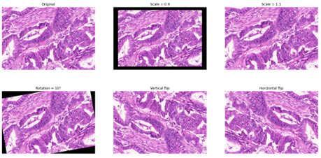
Some form of data augmentation is explicitly included in almost every method that were mentioned in this chapter, although the level of details on which operations are done vary wildly. Almost every method includes basic affine transformations, vertical and horizontal flips and random crops. It is also very common to include elastic distortions, random Gaussian blur or noise, scaling, or brightness/contrast variations (see Figure 3.6).
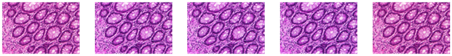
As mentioned above, colour data augmentation is also a common practice, often done in the HSV space (as in the example in Figure 3.7) or in a transformed, stain-specific colour space. For instance, “colour deconvolution” can be used to find each stain’s “colour vector,” which can then be used either to normalize the stains (by matching the stain’s vectors of an image to a reference target) or to perform realistic colour augmentation [67], [66]. While it is clear from challenge results and from other studies [66] that there is a very large consistent improvement in using basic morphological augmentation such as affine and elastic transforms over no data augmentation, the impact and importance of adding more complex augmentation methods is harder to assess and may depend a lot more on the specificities of a given dataset (e.g., from single or multiple source(s)) and application.
3.6.3 Network architectures
The results of digital pathology image analysis challenges and the evolution of the state-of-the-art make it very difficult to get to any sort of conclusion on which architecture(s) work best for which type of task. Some trends, however, can be noted. Until 2015, most challenges and publications focused on classification and detection tasks, and often used a classic classification macro-architecture, with several convolutional and max-pooling layers for feature extraction followed by some dense layers for discrimination. Those architectures are very close to the “pioneering” LeNet-5 and AlexNet, with some micro-architectural adaptations that the methods often do not really justify, nor systematically test their impact [51], [21], [6]. The main adaptation for the specificities of digital pathology problems come in the pre-treatment of the data, and the popularity of the “cascading” approach for highly imbalanced problems such as mitosis detection, as exemplified by Cireşan et al. [18] and Chen et al. [14] in their MITOS12, AMIDA13 and MITOS-ATYPIA-14 winning methods.
The situation slightly evolved after 2015 and the introduction of U-Net [58] and ResNet [33], which quickly became the standard “baseline” for segmentation and classification, respectively. As popular software libraries such as Tensorflow and PyTorch became available, so did open-source code for network architecture and even the weights of networks pre-trained on popular general-purpose datasets such as ImageNet. A standard approach to image analysis problems therefore became to start with a pretrained network and fine-tune it on the task-specific dataset. Digital pathology tasks, however, often require some additional tweaks, with many solutions adding multiple outputs (such as object borders and object inside [26], [72], [15]) or using ensemble of networks trained on subsets of the data, on multiple scales, or using different architectures [48]–[35]. In segmentation problems, however, our review noted that “when the methods are published with detailed results for the individual components, the improvement due to the ensemble over the best individual network is usually small (although ensemble methods do seem to perform consistently better, but generally without statistical validation)” [23].
Digital pathology detection problems appear to be challenging for classic detection networks such as Faster R-CNN or instance segmentation networks like Mask R-CNN, which need to either be included in an ensemble [48] or require significant post-processing [41].
In general, it seems that apart from very specifically designed networks such as HoVer-Net [26], very good results can generally be obtained with standard, off-the-shelf networks, with most domain-specific adaptations coming either in the pre- or post-processing stages.
Three different network architectures have been used (with some variations) in the different experimental works of this thesis. Their description can be found in Annex B, alongside those of the most commonly used networks in the literature.
3.6.4 Pre-training and training
As previously mentioned, many challenges top ranked methods use pre-trained networks, often from general-purpose datasets such as ImageNet, PASCAL VOC or ADE20K. Another option, used for instance by the winners of MoNuSAC 2020, is pretrain the network on data from similar datasets (from previous challenges, or other benchmark datasets).
In the methods analysed in our review, the training or re-training itself is generally done using the Adam optimizer (or some adaptation, such as the Rectified Adam), with the cross-entropy loss function or, alternatively, the “soft Dice” loss (or a combination of both).
To deal with the recurring problem of class imbalance, several methods have been proposed. One option is to weights the classes in the loss function so that errors on minority classes are more heavily penalized. Another is to use an adapted loss function such as the Focal Loss [45], which gives more weights to hard examples in the training set. A more direct approach is to balance the batches presented to the model by sampling the patches so that minority classes are “over-represented” compared to the actual distribution. Data augmentation can also be used to rebalance the dataset, by producing more “augmented” examples from the minority classes than from the majority classes.
3.6.5 Post-processing and task adaptation
Multi-outputs model typically require a post-processing step to put together the different parts of the results. A clear example of that can be found in the HoVer-Net model previously illustrated in Figure 3.4. The outputs of the “nuclear pixels prediction” branch are first combined with the outputs of the “horizontal and vertical map predictions” (which predict the vector to the centre of the nucleus) to compute an “energy landscape” and a set of markers that can be used to perform the watershed algorithm, thus providing the “instance segmentation.” The class of each segmented object is then determined by taking a majority vote from all per-pixel class prediction of the “nuclear type prediction” branch within the pixels of the object, to give the final “instance segmentation and classification.”
Another very common step is the stitching of patch predictions into a larger image, particularly for WSIs. In a classification task, this may take the form of a majority vote (where the WSI-level prediction is the majority vote of the per-patch prediction), but other task-specific rules may be used (for instance, in a grading problem, the final WSI grade may be the “worst”13 of the per-patch grades). In a segmentation task, an important choice is whether to include overlap or not in the tiling of the patches. If overlapping tiles are used, the final per-pixel prediction may be the majority vote of all patch predictions that included that pixel, but other heuristics may be applied. The fact that segmentation predictions tend to be worse close to the borders of a patch, for instance, may be used to weights the pixel prediction of a patch according to how close that pixel was to the centre of the patch.
3.7 The deep learning pipeline in digital pathology
With all these information in mind, we can now look at how the specific characteristics of digital pathology impact the deep learning pipeline that was presented in Chapter 1. Figure 3.8 illustrates the pipeline, and where the different elements that will be discussed in the rest of the thesis intervene.
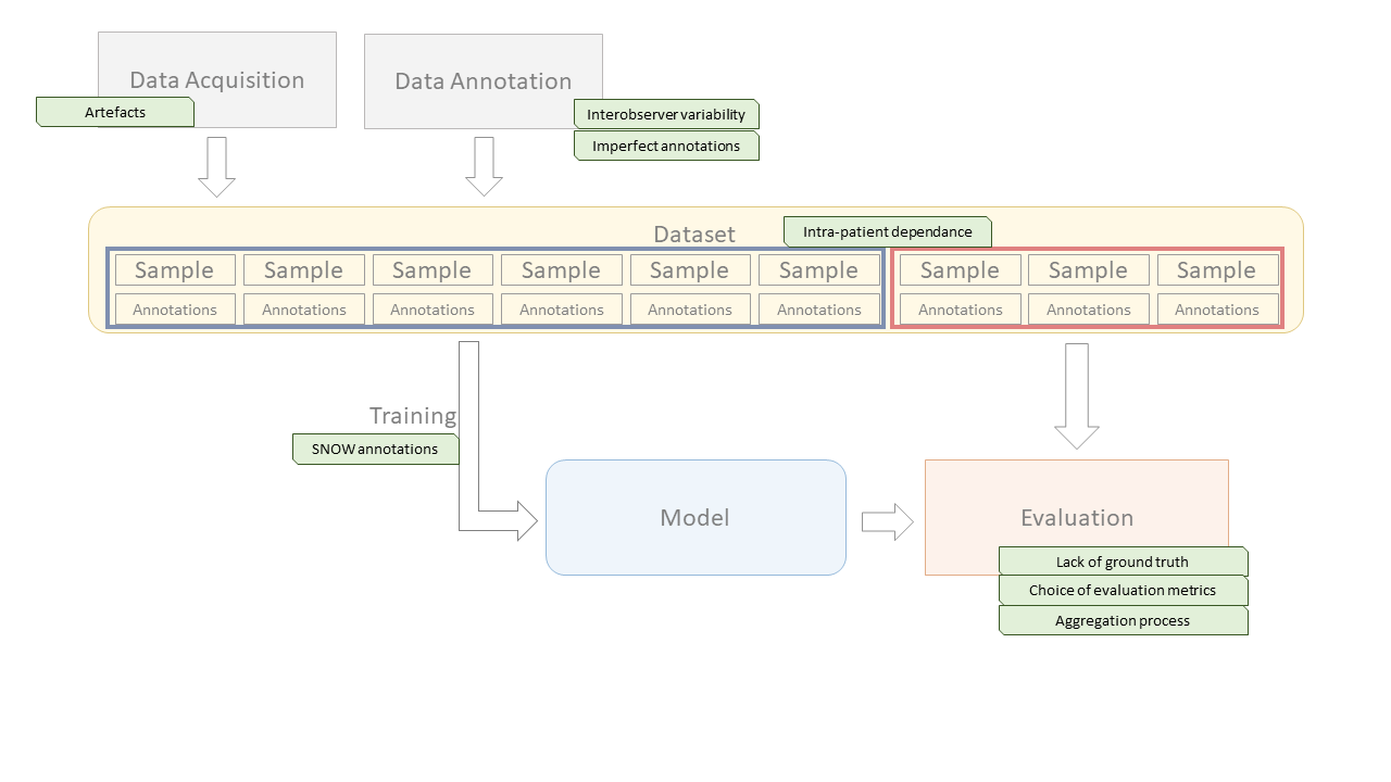
In Chapter 4, we will study the evaluation processes that are used, in challenges and in other publications, to assess the performances of deep learning algorithms. This includes not only the choice of evaluation metrics, but also the process of aggregating the results while considering the specificities of digital pathology datasets (such as the intra-patient dependence of samples), and the methods for ranking or otherwise comparing competing algorithms. We perform several experiments and theoretical analyses to better understand the biases of commonly used metrics, and the potential effects of class imbalance in classification and detection metrics.
In Chapter 5, we will investigate the question of how imperfect annotations affects the training process of deep learning model, through our SNOW (Semi-supervised, Noisy and/or Weak) framework. A practical example, the problem of artefact segmentation in whole-slide images, will be studied in Chapter 6. Artefacts that occur in the manipulation of the physical samples and in the acquisition of the images are very common in digital pathology. Segmenting these artefacts so that they can be safely removed from further automated methods, and so that the quality of the produced WSI can be objectively assessed, is a good practical example of the different challenging aspects of digital pathology datasets.
In Chapter 7, the more specific question of interobserver variability will be analyzed. Even if individual experts could provide their “perfect” annotations (meaning that the annotated samples perfectly correspond to their assessment of the images), the fact that individual experts would reach different assessments means that there can be no ground truth in a digital pathology task. This has an impact both on the training process, and on the evaluation process of deep learning algorithms.
Finally, in Chapter 8, we will study the question of quality control in challenges. This is transversal to the whole pipeline, as errors can occur anywhere from the constitution of the dataset to the evaluation process. Through the analysis of selected examples, we will examine the types of error that can undermine the trust that we can have on the results presented by challenges and provide some recommendations for future challenge organisers on how to ensure that the insights that can be gained from their efforts are maximized.
https://wiki.cancerimagingarchive.net/display/Public/Challenge+competitions↩︎
https://www.cancer.org/cancer/breast-cancer/understanding-a-breast-cancer-diagnosis/breast-cancer-her2-status.html↩︎
https://sites.google.com/view/nucls/data-generation?authuser=0↩︎
https://www.cancerimagingarchive.net/histopathology-imaging-on-tcia/↩︎
https://digitalpathologyassociation.org/whole-slide-imaging-repository↩︎
i.e. the highest one, as the grade is positively correlated with the malignancy level.↩︎