2. Digital pathology and computer vision

As we have seen previously, it is difficult to come to an entirely satisfying definition of deep learning. While the term “digital pathology” is not quite as fuzzy, it is still not entirely straightforward.

The 2014 Springer book “Digital Pathology” [40] defines it thusly:

Digital pathology, in its simplest form, is the conversion of the optical image of a classic pathologic slide into a digital image that can then be uploaded onto a computer for viewing.

They note, however, that “the concept and functionality of digital pathology has grown exponentially, so that a more accurate current definition would be that it is the field of anatomic and microanatomic pathology information systems,” including the “real-time evaluation, comparison, two- to three-dimensional reconstruction, archiving, dissemination for widespread viewing and consultation, compilation with other patient data, data mining, and use for education, clinical diagnosis and patient management, research, and the development of artificial intelligence tools [of specimens in digital form], and this may still only be scratching the surface.”

A 2010 Scientific American editorial [27] makes a graphical comparison between the pathway of “traditional pathology” and that of “digital pathology.” In traditional pathology, the slide is sent to the primary pathologist for “subjective analysis,” then “may be sent, in series by mail, to one or more consultants.” By contrast, in digital pathology, a slide is scanned and “screened by computer (objective analysis),” with the results attached to the patient electronic record so that “multiple reviewers can simultaneously see and discuss digitized slides and supporting documents.”

The Digital Pathology Association has the following definition:

Digital pathology is a dynamic, image-based environment that enables the acquisition, management and interpretation of pathology information generated from a digitized glass slide.¹

As can be seen from these definitions, digital pathology refers at the same time to the acquisition process of the optical information of the slide into a digital format, and to the different uses that can be made of the “virtual slide.” The main components of digital pathology can therefore be summed up as:

1. The acquisition hardware (slide scanner).
   
2. The visualisation software.
   
3. The “information system,” including the tools for sharing, distributing, and annotating the slides, and to link them to the rest of the patient records.
   
4. The image analysis software to automatically evaluate the content of the slide.

In this section, we will first briefly look at the history of computer-assisted pathology, from early attempts at automated pap smears analysis in the 1950s to the current era of deep learning and “grand challenges.” We will then look at the digital pathology workflow, and the needs that pathologists have for automated computer vision methods for research or clinical practice. Finally, we will take a snapshot of the digital pathology world in 2010, at the time of the first computer vision “challenge” in digital pathology, held at the ICPR conference, right before the Deep Learning “invasion.”

2.1 History of computer-assisted pathology

As digital pathology is an extension of traditional pathology, it is interesting to briefly look back at the history of computer-assisted pathology. The idea of using computers to automatically assess pathology samples is almost as old as computers themselves. If we want to look at the meeting of computer science and pathology, the best starting point might be 1955, with the presentation of the Cytoanalyzer by Walter Tolles [43] (shown in Figure 2.1).

The system is described as a scanner which converts “the density field of the slide into a serial electric current which is then used to analyse these several cell properties,” linked to a computer which function is to “accept the signal from the scanner, to apply certain rules of admission or rejection to the signals, to measure the desired cell characteristics and to distinguish between signals arising from abnormal cells and signals due to normal cells.” The results of clinical trials indicated that it was “inadequate for practical applications” [38], but the idea was interesting enough to lead to the development of similar instruments in the following years [39].

These early attempts at automated cytology have very limited “intelligence” and rely on very simple signal thresholding rules. This is understandable, given that they came before the founding of “artificial intelligence” as a field of computer science. Only a decade later, however, computer vision techniques were starting to take shape in cytology, with the development of the CYDAC to scan microscopic images, digitize them and convert them to magnetic tapes [28]. Automated computer vision methods to extract morphological information and determine cell types were developed by Mortimer Mendelsohn and Judith Prewitt in the mid-1960s [29], [36].

Around the same time, we find the first experiments in tele-pathology, with a Princeton laboratory mounting a black-and-white television camera on a light microscope [22]. The first clinical use of this technology would wait until 1968. A clinic at Logan International Airport in Boston was connected to the Massachusetts General Hospital in a very experimental telemedicine system which allowed pathologists in the hospital to remotely examine “black-and-white images of blood smears and urine samples using remote analogue video microscopy” [22]. The whole system was impressive in its scope. In addition to the video microscopy, it was equipped with “a range of cameras for long shots and close-ups to aid physical examination,” and other cameras for transmitting X-rays and electrocardiograms [12].

One of the pathology residents at the Massachusetts General Hospital at the time, Ronald Weinstein, would end up becoming one of the pioneers of modern tele-pathology in the 1980s, and was driven in part by the large interobserver variability among experts in clinical studies [49]. A big innovation that made tele-pathology more reliable was the introduction of “dynamic-robotic tele-pathology” (see Figure 2.2), allowing the remote observer to choose the field of view and focus of the microscope.

The dynamic-robotic tele-pathology of the 1980s required a pathologist “on hand” to remotely operate the microscope. When digital cameras became more readily available in the 1990s, systems with cameras mounted on a microscope taking static images and sharing them on a network of pathologist workstation became possible. However, these were unable to capture the entire slide. In 1999, however, Wetzel and Gilbertson introduced an automated whole-slide imaging system with 20x magnification and 0.33 µm/pixel resolution capable of imaging a slide in 5 to 10 minutes [18]. This did not immediately revolutionize the practice of pathology. In 2011, Pantanowitz et al [34] wrote that “there appear to be several technical and logistical barriers to be overcome before [Whole-Slide Imaging] becomes a widely accepted modality in the practice of Pathology,” citing the problem of artefacts such as tissue folds, bubbles and poor staining making the introduction of Whole-Slide Imaging (WSI) systems being shown “to stress the system in terms of reliability and throughput.”

As standardization of the process evolved and validation studies confirmed that digital pathology gave similar results to the “classical” methods, the regulatory framework evolved so that digital pathology started getting more readily adopted in clinical, research and educational practice [51].

The adoption of WSI had a huge impact on image analysis for pathology, with entire slides being now available for analysis instead of limited fields of view [10]. Larger datasets could now be gathered and provided to the image analysis and artificial intelligence community, leading to the development of algorithms that promised to “improve accuracy, reliability, specificity and productivity” of digital pathology [33]. As with deep learning, the development of new software tools such as the “vendor-neutral” OpenSlide library [37] has made the programmatic use of WSIs easier, allowing more researchers to design image analysis pipelines.

2.2 The digital pathology workflow

The digital pathology workflow is a long, multi-steps process that requires trained specialists and specialized hardware. In this section, we will look at those steps, from the extraction of the tissue samples from the patient to several uses of the digitized images.

2.2.1 Sample acquisition: from the body to the scanner

Tissue samples can be acquired from the patient during surgeries or biopsies. After extraction, a sample will go to a series of tissue processing steps [50]: fixation, dehydration, clearing, paraffin infiltration and embedding. The goal of these steps is to stabilize the tissue and to create a “block” that can be sectioned with minimal damage. The block can then be cut into thin slices (around 5 µm) using a microtome, which are then mounted onto glass slides.

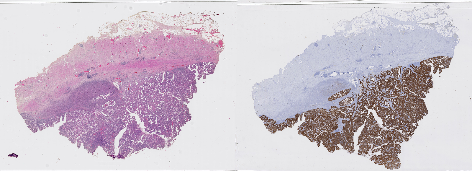
The next important step is the staining of the tissue. Staining techniques were developed as early as the mid-nineteenth century [42]. Staining agents will selectively stain certain tissue components, creating contrasts that allow the pathologist to better see the structure of the tissue. The mechanisms through which certain stains will favour certain tissue components are complex, relying on different biochemical processes [19]. The most widely used general-purpose stains combination is haematoxylin combined with eosin (H&E). Essentially, haematoxylin stains nuclei in blue, eosin stains cytoplasm and extracellular matrix in pink. More recently, immunohistochemical (IHC) techniques have been developed to selectively reveal the expression of target proteins in the tissue, using antigen-antibody interactions. Figure 2.3 shows two whole-slide images from the same tissue block, stained with H&E and using an IHC marker, respectively.

Once the slide is ready, it can go through the scanning process to be digitized. Slide scanners are essentially optical microscopes combined with a digital image capture device, and a mechanical system to change the acquired region. WSIs may be obtained using a line scanning process (with the camera capturing strips) or a tile scanning process (with the camera capturing squares) [3]. The highest resolution available is generally ‘x20 equivalent’ (around 0.5µm per pixel) or ‘x40 equivalent’ (0.25µm per pixel). The main challenges of the scanning process are the stitching of the lines or tiles, and the management of the focus over the whole slide, as the focal plane will vary with the topography of the tissue section.

As an alternative to the WSIs produced by this workflow, it is also possible to put multiple small tissue samples extracted from different patients on the same block to produce “tissue microarrays” (TMA). While WSIs have the advantage of providing more context by showing large regions of tissue, TMAs make it possible to process more samples more quickly and homogeneously.

2.2.2 Applications

The first, and probably most common application of digital pathology is telepathology. Digitized “virtual” slides can be sent to pathologists outside of the facility where the samples were acquired. This allows for a greater specialization of the pathologists and makes it easier to get second opinions for difficult cases [40].

More interesting to us in the context of this thesis are the applications related to image analysis. It is particularly important to understand what pathologists hope to get from computer vision algorithms, as there can sometimes be a disconnect between the needs of pathologists and the products of the machine learning and computer vision communities [17].

Hamilton et al. list some “key areas where image analysis has had a role to play in pathology and tissue-based research” in 2014 [16]:

• Quantitative evaluation of nuclei (morphology, DNA content…)
• Measures related to tissue architecture (e.g. cellular organisation)
• Quantitative immunohistochemistry and biomarker discovery
• Tissue microarray analysis
• Measure of tumour heterogeneity
• Measures of fluorescence properties
• Automated tumour detection

In general, the main expected improvement of using automated methods is to avoid the problems of “inconsistency in diagnostic decision-making in pathology, poor reproducibility in grading disease and the variation that exists in image interpretation.”

Madabhushi and Lee provide a review of image analysis and machine learning in digital pathology in 2016 [26]. The first big research avenue they identify is “segmentation and detection of histologic primitives,” such as glands and nuclei. They see this as an important prerequisite for quantitative histomorphometry, the detailed characterization of the morphologic landscape of the tissue. Another direction for image analysis is “tissue classification, grading and precision medicine.”

These applications may be used as aid to clinical diagnosis, but also for research purposes: as the digitization of pathological slides becomes routine practice, huge datasets can be created, and automated measures may be extracted for large retrospective studies.

2.2.3 Cancer grading systems

Cancer staging or grading systems provide a codification of the assessment of a tumour, which is useful to provide prognosis (i.e. cancer outcome prediction, such as risk of recurrence after treatment or death) and to compare groups of patients [6].

The Tumour-Node-Metastasis (TNM) system, maintained by the American Joint Committee on Cancer (AJCC) and the International Union for Cancer Control (UICC) is the “general purpose” tumour grading system, in the absence of another system specifically targeted to the cancer type. The grades are based on an aggregation of three categorical assessments [11]:

• The Primary Tumour category, based on its size and extent. Categories generally include TX (unknown), T0 (no evidence of primary tumour), Tis (in situ carcinoma), T1-T4 (primary invasive tumour, with higher categories based on size and/or local extension).
• The Regional Lymph Node category, assessing the existence and extent of a regional lymph node involvement. Categories generally include NX (unknown), N0 (no regional lymph node involvement), N1-N3 (regional node(s) containing cancer cells, with higher categories for increasing number of nodes, size of the nodal cancer deposit, etc.)
• The Distant Metastasis category, which specifies whether there is evidence for the presence of distant metastasis (M1) or not (M0) at the time of diagnosis.

It is important to note that the histopathological examination of the tumour is only a part of the grading criteria, alongside other imaging modalities, physical examination, clinical history, etc. While there are general criteria and trends that are common in all cases, the specific staging is tuned to the specific tumour types based on relevant survival studies.

For some cancer types, alternative systems have been fully validated and are now largely adopted worldwide [11], including the Gleason scoring system [13] for prostate cancer (and its 2016 Epstein modification [8]) and the Nottingham system [7] for breast cancer.

The Nottingham system is based on the assessment of tubule formation (with three categories based on their extent relative to the total tumour), nuclear pleomorphism (three categories based on the size and regularity of the nuclei) and mitotic count (three categories with specific numbers depending on the examined field area).

The Gleason system is based on a “relatively low magnification” assessment of the pattern of growth of the tumour, with five distinct pattern types of increasing apparent malignancy being identified (see Figure 2.4). The predominant (“primary”) pattern and lesser (“secondary”) pattern are recorder for each case, and the final score is based on the addition of the two pattern categories (so if the “pattern 3” is predominant with some “pattern 2” present, the score would be 3+2 = 5).

These two systems in particular have driven a lot of research in computer vision for digital pathology, as their criteria are directly based on the analysis of the pathology samples. It is therefore not surprising that lots of publications and challenges relate to nuclear detection and segmentation, mitosis detection, or Gleason scoring.

2.2.4 Immunohistochemistry (IHC)

Immunohistochemistry use antigen-antibody interactions to selectively bind the staining agent to target proteins. This allows for a specific targeting of cells that express those proteins. By carefully selecting the antibodies, it is therefore possible to discriminate between the benign and malign nature of certain cell proliferations, or to identify micro-organisms or materials secreted by cells [5].

IHC techniques can therefore be extremely useful at the clinical level for diagnosis. It is also very valuable from a research perspective, in the search of biomarkers that may or may not correlate with tumour aggressiveness or patient outcome. The interpretation of IHC images, however, can be very difficult and subjective, often based around an estimation of the proportion of tissue or cells where the stain is present, leading to large inter- and intra-observer variability [48].

The overall structure of the cellular tissue is usually made visible through a “counterstain” (often haematoxylin) which makes all the cells visible (see Figure 2.3).

2.3 Image analysis in digital pathology, before deep learning

As we will show in the next chapter, deep learning techniques quickly spread in histopathological image analysis in the 2010s. Before we get to those algorithms, however, it is interesting to take a look at what existed before.

In 2009, Gurcan et al. published a large review of histopathological image analysis [15]. The next year, they organised the ICPR 2010 “Pattern Recognition in Histopathological Image Analysis” (PR in HIMA) challenge, where several image analysis algorithms were tested on lymphocyte segmentation on breast cancer images, and centroblasts detection in follicular lymphoma [14].

A 2011 review by Fuchs et al. [9] also provide some interesting insights on the state of “computational pathology” at the time, with a particular focus on questions of interobserver variability and ground truth generation which will be discussed more fully in later chapters of this thesis.

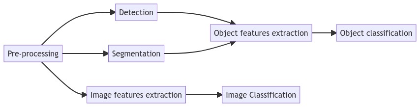
From these reviews, we can see how the classic image analysis pipeline (presented in Figure 2.5) has been adapted for digital pathology.

2.3.1 Pre-processing

The interpretation of histopathological images relies a lot on the staining process. A very common pre-processing step in digital pathology image analysis consists in stain or colour normalisation. The objective of this step is to reduce the differences due to the exact protocol used for the staining process, or to differences in the acquisition setup or the acquisition hardware. For instance, Figure 2.6 illustrates how the same slide scanned by two different machines can lead to large differences in the colours of the resulting digital images.

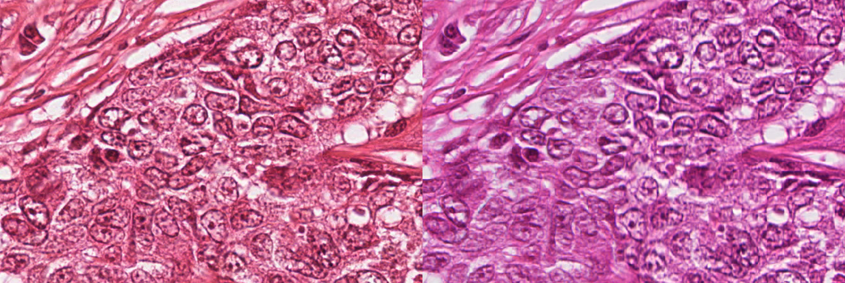
Typically, stain normalization methods are based on the knowledge that, in general, histopathological slides use a combination of two stains. The most common combination is H&E, where the blue haematoxylin stains the nuclei, and the pink-red eosin stains the cytoplasmic elements [42], whereas in immunohistochemistry there is generally a combination of an IHC marker, often using 3,3’-Diaminobenzidine (DAB) as chromogen which exhibits a brown colour, with a haematoxylin counterstain. In 2009, Macenko et al. [25] proposed to look at the pixel distribution in the RGB colour space and to use Singular Value Decomposition to find the two main directions of the distribution. Colour deconvolution [47] can then be performed to separate the contributions to the two “stain” channels, and colour normalization consists in aligning the vectors of the “target” image to the vectors of a “reference” image. Several improvements on the same general concept have been proposed over the years, as stain normalisation is still often used as a pre-processing step even with deep learning techniques [45], [44].

Another important characteristic of histopathological images is their size. It is not uncommon for WSIs to have a full resolution size of around 80.000x60.000px, taking up about 15 gigabytes of data.² Even with today’s hardware, it is impractical to apply any image analysis algorithm to the entire slide at once. A typical pre-processing step would therefore consist in extracting image patches from the larger WSI. If the entire WSI is to be processed, then a common strategy would be to use a regular tiling grid on the image to extract evenly spread patches that cover the whole slide. As a large part of the slide will often only contain the glass slide itself and no tissue (see Figure 2.3), a simple thresholding method can be applied to filter empty patches.

2.3.2 Detection and segmentation

While detection and segmentation are often “end goals” of computer vision methods by themselves, they generally are not the desired outcome for pathologists, but rather an important step towards disease grading or diagnosis [15]. However, as fully automated diagnosis systems are even today largely out of reach (and arguably not particularly desirable in the first place), detection and segmentation results still hold a lot of interest. In clinical practice, such applications may for instance provide pathologists with measures such as cell counts or mitotic counts, which are very time consuming for human experts to provide and obvious candidates for automatization.

Nuclei segmentation has been the subject of a lot of research. While it seems at first glance that relatively simple thresholding techniques may give good results, as the nuclei are typically much darker than their surroundings (see Figure 2.7), the large variability in image sets leads to inconsistent results [15]. Watershed-based methods suffer from the same issues. Doyle et al. [30] proposed a slightly more complex method. A first thresholding is made to keep all low intensity pixels. It is followed by a Euclidian Distance Transform (EDT) to compute the distance to the closest background pixels. Another threshold is applied to the EDT results to keep pixels that are far from the background (and therefore should be closer to the centre of the objects of interest), and template matching with different elliptical templates representing usual nuclei shapes and sizes is then applied and pixels with a high correlation to at least one of the templates are kept as “nuclear centroids.”

Similar pipelines were developed for gland segmentation, where first low-level colour and texture information are used to give a general pre-classification of each pixel, then further constraints based on shape, size and spatial relationships are used to refine the results [15].

2.3.3 Feature extraction

Feature extraction is where domain knowledge particularly needs to be present in classic image analysis pipelines, as the useful features are often inspired by the attributes identified by pathologists as relevant for grading and diagnosis.

Object-level features are computed on the pixels that intersect with the binary mask of the previously segmented object. They include information about the shape and size (area, eccentricity, perimeter, centre of mass, symmetrical properties…), the colour information (optical density, hue…), or the texture (co-occurrence matrix features, wavelet features…) [15].

Colour and texture-based features can also be extracted directly on full images or image regions to provide patch-level classification. Another approach to use the detected object is to build a graph of their spatial relationship across the entire image, and to then compute graph-based features to characterize these relationships [2].

It is also common to use a multi-resolution approach to compute those features, especially if working with larger WSI images, as they tend to contain different types of information at different scales, from the very high-resolution nuclei to larger tissue structures such as glands.

2.3.4 Feature selection and classification

Long before deep learning methods were applied, machine learning approaches were already used to perform classification based on the extracted features. While many algorithms in the 2000s mostly relied on rule-based expert systems, it was also very common to see a more statistical approach to pattern recognition [9].

The machine learning approach to pattern recognition consists in computing as many independent features as possible in the feature extraction phase, then to reduce the dimensionality of the problem based on the information present in the dataset. For instance, features can be added or removed from the feature set based on whether their presence improves the classifier. Dimensionality reduction can also be done using statistical methods such as Principal Component Analysis (PCA), transforming the feature space so that its dimensions are as informative to the classifier as possible.

In terms of the classifiers themselves, the most popular in the 2000s in digital pathology image analysis were probably the Support Vector Machines (SVMs). It was also established that ensemble classifiers were, in general, the preferred solution to reduce the bias and variance of individual classifiers [15].

2.3.5 Methods from the ICPR 2010 PR in HIMA competition

These different approaches are well illustrated by the methods proposed by two participating teams at the ICPR 2010 PR in HIMA competition for lymphocyte segmentation. Their overall pipelines are illustrated side-by-side in Figure 2.8.

In Kuse et al. [23], a pre-processing is applied to reduce the number of colours in the image using a mean-shift clustering. A thresholding operation is then done based on the Hue value in HSV space to find candidate nuclei. The candidates are labelled using connected components analysis, and a contour-based approach is used to separate overlapping nuclei. Eighteen texture features were extracted and used to train a SVM classifier on a supervised set of lymphocyte / non-lymphocyte nuclei.

Meanwhile, Panagiotakis et al. [32] first reduced the dimensionality of the image by performing a PCA in colour space and selecting the first dimension. A Mixture of Gaussian model was then used to determine three separate pixel values distributions representing stroma, non-lymphocyte nuclei and lymphocyte nuclei. Regions detected as candidate nuclei are filtered based on handcrafted area and eccentricity criteria. Two features are then extracted from each remaining candidate region (mean value and variance), and a Transferable Belief Model filters out remaining non-lymphocytes. Finally, the area and eccentricity are used again to split overlapping nuclei in an iterative method that tries to maximize a criterion describing the “expected shape” of the objects.

2.3.6 Mitosis detection

Mitotic count is often used as part of the grading system for different types of cancer [11], such as with the Nottingham system used for grading breast cancer tumours [7]. The development of automated counting, detection or segmentation methods has therefore been a topic of interest for some time. Figure 2.9 illustrates the pipelines of several methods proposed over the years.

Between 1984 and 1997, a Dutch team developed and improved a mitosis detection method using a “classic” image analysis pipeline [1], [21], [41]. Their first attempt used greyscale photographs of microscopic images. They selected candidate nuclei based on simple thresholding and morphological filtering. Linear discriminant analysis was then used on some contour and histogram features to classify the candidate between mitosis and non-mitosis. Over the years, they improved the method by obtaining better acquisition devices, moving to colour images (and therefore colour features), and using a region growing approach to select the candidate nuclei. While their False Positive Rate remained relatively high (22-42%), they concluded that the false negatives were rare enough (5-8%) that “the current system may serve well as a pre-screening device” [1].

Progress, however, was slow. The 2008 method by Dalle et al. [4] is not that different from the 1997 attempt by Beliën et al. They used global thresholding and morphological filtering to detect candidate nuclei, and then a Gaussian model to discriminate between mitotic and non-mitotic cells based on a few shape and colour features. The main difference of Dalle et al.’s method is that they go one step further in the “automated diagnosis,” as they compute the mitotic score (three categories based on the mitotic count) and evaluate their method based on the agreement on the score with a pathologist, instead of the per-mitosis detection performance. While it is certainly interesting to get closer to a clinical application, it is also difficult to compare their performance to other methods as they do not provide any per-mitosis results.

Classic pipelines for mitosis detection did not entirely disappear after the start of the deep learning era. In 2015, Paul et al. [35] claimed state-of-the-art results on several mitosis detection challenge datasets (MITOS12, AMIDA13, MITOS-ATYPIA-14) without deep learning. In their pipeline, they first use only the red channel for pre-processing and the segmentation of candidate nuclei. They then use the red and green channel normalized histograms of the candidates with a random forest classifier to discriminate between mitosis and non-mitosis. The selection of candidate nuclei in Paul et al. is significantly more complex than in the previous methods, with an iterative entropy-based pre-processing and segmentation step, and the Random Forest classifier is able to manage the higher dimensionality of the very low-level features computed.

2.4 Characteristic of histopathological image analysis problems

To conclude this chapter, we will summarize the main characteristics of histopathological image analysis problems.

2.4.1 Colour spaces

Modern whole-slide image scanners produce colour images encoded with either 8-bits or 16-bits RGB channels. The distribution of the pixels in the colour space is very different from what can be found in natural images (such as photographs, for instance). The staining process used in the preparation of the tissue sample means that there will generally be few distinct hues in the image, as illustrated in Figure 2.10. As we previously mentioned, pre-processing steps such as stain normalisation or deconvolution are very common in digital pathology image analysis pipelines.

2.4.2 Image size and multi-scale information

WSIs are very large images. At full resolution, they can take gigabytes of disk space, and therefore cannot be processed all at once. WSI scanners can acquire the image at different levels of magnification. It is therefore possible to use multi-scale information not just from interpolation to lower resolutions (with the risk of aliasing artefacts), but also by switching between the different acquisition magnification levels. Histopathological image analysis pipelines have to determine which resolution, or resolutions, contain the information needed to solve the task. Some tasks, such as mitosis detection, typically work better at the highest resolutions available, so that nuclei features are visible [1], but for other applications such as Gleason grading it may be beneficial to use lower magnification levels (which implies seeing a larger context in a same-sized patch) to detect useful features [31].

2.4.3 Scope and explainability

In digital pathology, the scope of the problem is generally much larger than the specific image analysis task that the algorithm is trying to solve. The output of an image analysis system will typically be either an image-level assessment (class, grade…), an object-level assessment (count, localisation…) or a pixel-level assessment (segmentation). The expected output of a fully automated “AI for digital pathology” system, however, would be a patient-level diagnosis or prognosis or therapy indication, and would have to incorporate data outside of the image into its inputs (such as patient history, other imaging modalities, laboratory data, etc. [24]). The potential trap of a direct data-to-diagnosis approach, however, would be to create a “black box” effect where it becomes impossible (or at the very least impractical) to determine the “reasoning” behind an algorithm’s output.

Intermediate, lower-level outputs such as those typical in image analysis problems are therefore still very relevant to produce, as they provide the potential for better explainability of the algorithms’ results. The clinical end result, however, should not be forgotten either. It should at the very least inform the evaluation process and metrics by which the results on a task should be assessed.

The criteria for object classification or tumour assessment are often fuzzy and ill-defined. Despite great efforts to standardise and objectify these criteria, there is still often a lot of room left for the subjective (and experienced) view of the pathologist. This also makes it hard to describe the image analysis tasks formally, and to design expert rules. Digital pathology tasks are therefore good candidates for deep learning methods, which are capable of designing their own features directly from the data. The acquisition and annotation of the data, however, is very challenging for the same reasons, and obtaining accurate supervision is, as we will see in the rest of this thesis, a constant struggle and one of the largest issues that deep learning faces in digital pathology.

2.4.4 Classification and scoring

In many digital pathology classification tasks, the categories are ordered. As we have seen, many tumour assessment standards revolve around “scores” or “grades.” These problems are therefore straddling the line between “classification” and “regression.” However, even though they are ordered, they are typically treated as distinct categories. We will generally refer to these sorts of tasks as scoring tasks, which can be seen as a subcategory of classification tasks.