---- 8.1 MITOS12: dataset management
---- 8.2 Gleason 2019: annotation errors and evaluation uncertainty
---- 8.3 MoNUSAC 2020: errors in the evaluation code
------ 8.3.1 Error in the Detection Quality computation
------ 8.3.2 Undetected false positives
------ 8.3.3 Aggregation strategy
------ 8.3.4 Error in the reporting of the per-class results
------ 8.3.5 Corrections and scientific publishing
---- 8.4 Discussion and recommendations: reproducibility and trust
8. Quality control in challenges
The organisation of digital pathology challenges is a very complex process that is inevitably subject to errors. These errors can happen anywhere from the annotation process to the evaluation code or the analysis of the results. They can also significantly impact the results of the challenge, and therefore the conclusions drawn from them, influencing the trends in designing models and algorithms to solve similar tasks in the future.
In this chapter, some examples of mistakes in challenges will be examined. More specifically, our focus will be on the problems that those mistakes can cause during and after the challenge, and what can be done to mitigate those effects. The three main challenges that will be used as examples are the MITOS 2012, Gleason 2019 and MoNuSAC 2020 challenges. We already mentioned the main issues with the MITOS 2012 challenge, which were examined by Elisabeth Gruwé in her Master Thesis [4] and acknowledged by the organisers in the post-challenge publication [16]. Some of the problems of the Gleason 2019 challenge were reported by Khani et al [7] in 2019, and we added our own analysis in different publications [2], [1]. Our analysis of the MoNuSAC 2020 errors were published as a “comment article” in response to the challenge’s publication [3], alongside the author’s response [18], while some additional analyses were provided in a research blog publication[^54].
It is important to emphasize here that these analyses should not be taken as a condemnation of the challenge organisers. Part of the reason that we were able to conduct these analyses is because the challenges were more open and transparent about their process than most. The MITOS12 challenge organisers, for instance, published their full test set annotations, organized one of the first digital pathology challenges, and corrected most of their problems by the time they organised the 2014 edition of their challenge, MITOS-ATYPIA 14. Gleason 2019, as we have established in the previous chapter, is the only digital pathology challenge to publish multiple individual expert annotations, allowing for a much finer analysis of interobserver variability than what is usually possible. MoNuSAC 2020, meanwhile, is the only digital pathology challenge to publish the predictions of some of the participating teams on the whole test set, instead of the summarized result metrics and selected examples for the post-challenge publication. This alone makes it a very valuable resource, despite the problems with the results of the challenge themselves.
8.1 MITOS12: dataset management
Mitosis detection, as we have seen through this thesis, has been a very popular topic for image analysis. The ICPR 2012 Mitosis Detection challenge was very influential in opening up the field of digital pathology to deep learning methods, thanks to the excellent performance obtained by the IDSIA team of Cireşan et al. The dataset was made out of selected regions from five H&E-stained slides, each coming from a different patient. Each slide was scanned with three different whole-slide scanners. Ten regions per slide were selected, and they were split into a training set of 35 regions and a test set of 15 regions. The annotations were made by a single pathologist, who annotated 326 mitoses.
The detection task evaluated in the challenge consisted in predicting the centroids of the mitosis. A predicted mitosis was determined to be a “true positive” if its centroid was within a range of 5µm from the centroid of a ground truth mitosis. The Precision, Recall and F1-Score were used as metrics, with the F1-Score being the primary measure for the ranking[^55].
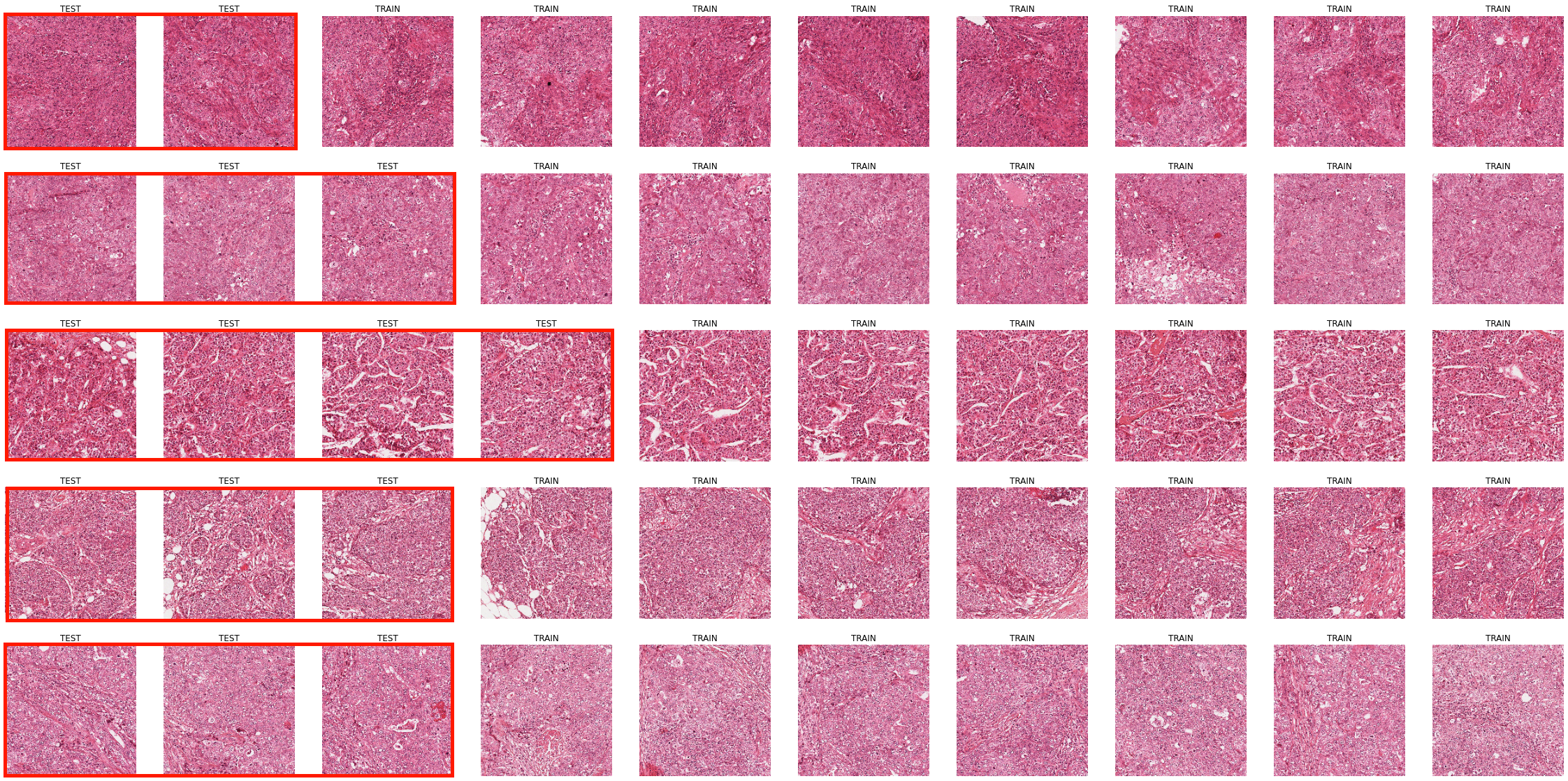
The use of a single pathologist for determining the ground truth is an obvious limitation of the dataset, but the most important problem is clearly that the dataset is split at the image region level instead of at the WSI level (which in this case is the same as the patient level). All the image regions from the dataset are shown in Figure 8.1, with the test set images framed in red. It is clear, even looking from a very low-resolution point of view, that images extracted from the same patients will share common features.
In Gruwé’s Master Thesis [4], a comparative study was made between evaluating with a five-fold cross-validation with the split at the image level, with a five-fold cross-validation at the WSI level (which in this case corresponds to a “leave-one-patient-out” cross-validation). With the image level cross-validation, the average F1-Score obtained was 0.68, whereas for the leave-one-patient-out cross-validation, it was 0.54.
It is clear that keeping the test set as independent as possible from the training set should be standard practice to avoid learning patient-specific features. However, as public challenge datasets attract researchers which may not be familiar with the specificities of biomedical data, splits at the image level can still be found in recent publications. For instance, Rehman et al. [15] demonstrate excellent results on the four usual mitosis datasets (MITOS12, AMIDA13, MITOS-ATYPIA-14 and TUPAC16), but their experimental setup was that “[e]ach dataset was divided into five chunks each containing 20% randomly selected images of the dataset.” In doing so, they actually propagate the “mistake” of the MITOS12 dataset to the later datasets where the challenge split was correctly made. A similar error is done in Nateghi et al. [9], where “each dataset is divided into five random subsets and 5-fold cross-validation is performed in each of these subsets,” with the MITOS12, AMIDA13 and MITOS-ATYPIA-14 datasets being used.
A key factor in this reoccurring error may be the unavailability of the test set annotations for the later challenges, even years after the end of the competition. Researchers thus have to make their own train/test split from the available training data, which can easily lead to them overlooking some key aspects of the methodology. This in turns leads to improper comparisons between methods, made on different subsets of the data.
8.2 Gleason 2019: annotation errors and evaluation uncertainty
The Gleason 2019 publicly released training dataset contains 244 H&E-stained TMA cores annotated by 3 to 6 expert pathologists (see Annex B). These maps show a large variability between the experts, which is expected given the high interobserver variability typically observer for that task. Part of the variability, however, is not just due to differences of opinions, but to clear mistakes in the creation of the annotation maps from the expert annotations. These mistakes were first noted by Khani et al. [7], who noted that “some of the contours drawn by the pathologists were not completely closed,” which led to the corresponding regions not being filled in the annotations. Some examples are shown in Figure 8.2. For their own experiments, Khani et al. identified and manually corrected 162 of these problematic annotation maps. From our own analysis, several more annotation maps with mistakes were identified, bringing the total to 185 of the 1171 available annotations, meaning that around 15% of the provided annotation maps are incorrect.

These mistakes are also not randomly distributed in the dataset, as some experts are largely more affected than others, as shown in Table 8.1. Pathologist 2 is particularly affected by this problem. Taking a more detailed look at the annotations show that, in general, this pathologist attempted to be a lot more detailed in their annotations compared to the others. In our own experiments on interobserver variability presented in Chapter 6, we chose to remove those annotations from the dataset instead of potentially adding our own biases and mistakes by attempting a manual correction.
| Pathologist 1 | Pathologist 2 | Pathologist 3 | Pathologist 4 | Pathologist 5 | Pathologist 6 |
|---|---|---|---|---|---|
| 5 | 119 | 54 | 6 | 0 | 1 |
It is unclear whether these problems are also present in the test set used by the challenge, as those annotations were not made public. Other publications using the same dataset make no mention of these mistakes [14]–[8]. The dataset used by the challenge’s organizing team in their publications [5], [11], [12], [6] does not seem affected by those mistakes, which suggests that they may have happened during the process to generate the data files for the challenge itself. An example of clear differences between the annotations from the challenge organizers’ publications and those found in the public dataset is shown in Figure 8.3. Unfortunately, the challenge organizers did not respond to our requests for clarification to the contact address provided on the challenge website. One contacted author of subsequent studies responded that he agreed “that the data uploaded on the challenge website has the problem that you indicated,” without elaborating further.
![Figure 8.3. Difference in the annotation map for “Pathologist 2” on a TMA core between an illustration from Nir, 2018 [11], and the publicly available annotation map from the challenge website[^56] (“slide005_core063”). In addition to the “closed contour” difference, some details from the publicly released dataset are missing from the one used by Nir et al., such as some detailed indentations in the contour (solid black arrow), or some smaller annotated regions (dotted black arrow).](./fig/8-3.png)
The evaluation of the challenge also shows some signs of potential issues. The results reported on the challenge’s website include a ranking of all the teams based on a custom score which combines the Cohen’s kappa, the micro-averaged F1-Score and the macro-averaged F1-Score. They also provide a confusion matrix of the pixel grading for each of the top 8 teams, which is announced as being normalised so that each row (representing the "ground truth" grade) sums up to 1, providing the sensitivity of each grade on the diagonal. There is no available evaluation code, and the exact definition of the metric is unclear (Cohen’s kappa could be unweighted, linear or quadratic, the F1 score could be computed on the image-level classification task or on the pixel-level segmentation task, and the macro-averaging could be done as the arithmetic mean of the per-class scores or as the harmonic mean of the average precision and recall). In any case, the values presented on the challenge website[^57] for the confusion matrices have some inconsistencies, as illustrated in Figure 8.4. Many rows do not sum up to 1, with differences that cannot possibly be explained by rounding errors. Some of the results, such as for the algorithms ranked 5th and 7th in Figure 8.4, imply that no predictions for Grade 5 were made at all.
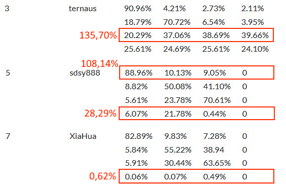
As the evaluation code is not available, there is no way to know if the errors were only made in the reporting of the results on the website, or if they impacted the final score on which the rankings were made. They also appear in the recently released post-challenge publication of the challenge winners [13], in which the and both F1-scores are used for the pixel-level evaluation, and accuracy, precision, sensitivity and specificity are used for the core-level evaluation. Confusingly, the reported individual components of the challenge metric (i.e. , and ) do not match with the reported score using the formula provided by the challenge organizers. As of June 2022, no official “challenge” publication has been made (in fact, none of the publications by the University of British Columbia team refer to the competition itself), making it very difficult to fully understand the exact evaluation process.
8.3 MoNUSAC 2020: errors in the evaluation code
The MoNuSAC 2020 challenge was remarkably transparent about their data, the results of the participant, and their code. A pre-challenge preprint was published on ResearchGate[^58] detailing the challenge procude, the evaluation metric, and the expected submission format. Code for reading the annotations and for computing the evaluation metric was released on GitHub[^59]. Examples of the submission file’s format were provided via Google Drive[^60]. After the challenge, in addition to the post-challenge official publication [17], supplementary materials were released with all of the participating teams’ submitted methods[^61].
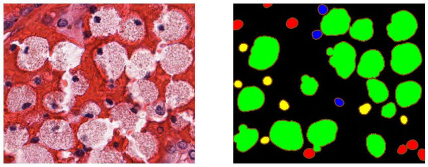
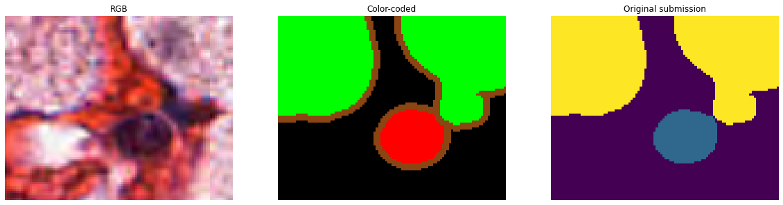
All the images and annotations from the training and the test set were also released on the challenge website[^62], as well as the “color-coded […] predictions of top five teams.” These “color-coded” predictions were not the raw submissions of the challenge participants, but a visualization that emphasized the contours of the segmented objects (as shown in Figure 8.5). As the challenge’s task is instance segmentation and classification of cell nuclei, being able to visually assess the separation between objects is important. The ground truth annotations were provided as XML files with the vertex position of all annotated objects.
Providing the teams’ predictions, the ground truth and the evaluation code should in theory be sufficient for independent researchers to reproduce the results of the challenge. Several issues make that reproduction difficult in this case. First, the “color-coding” process makes it difficult to recover the exact pixel-precise predictions of the participating team. Thanks to the collaboration of Dr. Amirreza Mahbod, who kindly shared with us the raw submission files of his team, we can see that this visualization was made by adding a 3px wide border outside of the predicted object (see Figure 8.6). For relatively isolated object, it is therefore possible to automatically recover the teams’ predictions from the color-coded masks. However, for objects that are close together (frequent in cell nuclei segmentation), this coding introduces uncertainty on the exact boundary between objects due to thickened contours that create artefactual overlaps (see Figure 8.6). Second, a careful analysis of the public evaluation code shows that it had to use more than the publicly released ground truth annotations and evaluation code. The code that reads the XML annotation files[^63] produces TIF image files (one file per nucleus class and per RGB image), whereas the code that computes the Panoptic Quality evaluation metric[^64] reads the ground truth from MATLAB files, which was the required format for the participants submissions.
These are, however, relatively minor problems, and the results of the challenge should still be reproducible from the available data, within a reasonable range of error. The evaluation code itself, however, contains several mistakes that make the published results highly unreliable. Our analysis of these errors was published as a comment article to the challenge publication [3]. In this section, we will present our analysis and the author’s reply [18].
8.3.1 Error in the Detection Quality computation
The Panoptic Quality, as we previously established in Chapter 4, section 4.4.8, combines the “detection quality” (with the F1-Score) and the “segmentation quality” (with the average of the true positive objects). In MoNuSAC, these values are aggregated by first computing the (per-image and class ), then computing the average per-image , where is the number of classes in image . Finally, the average on the whole test set is computed as , with the number of images in the test set.
In the provided code, this is done in the “PQ_metric.ipynb” notebook available on the challenge’s GitHub. The method Panoptic_quality(ground_truth_image, predicted_image) computes the . It takes as input the ground truth "n-ary mask" (i.e. the mask of labelled objects in the class) and the predicted n-ary mask. Some regions from the images were also marked as “ambiguous” in the ground truth annotations and were thus removed from the ground truth and the predicted images before computing the metric. This method, however, contains a bug, which is detailed in our analysis available on GitHub[^65].
The error causes the list of “false positives” in the image to be overestimated in some cases. The effect of the error can be very different depending on the strategy used by the team to generate the instance number in the “n-ary masks.” Indeed, there are two strategies when generating the per-class prediction masks. As each class prediction has to be sent separately, it makes sense to reset the instance count for each class, so that the "n-ary mask" will always start with instance index 1. Conversely, as the goal of the challenge is to provide "segmentation and classification" for all classes in an image, it would also make sense to provide a unique instance number for each object in the image, and then to separate the objects by class. In that case, the instance indices could follow each other from class to class (for instance: [1,2, ..., N] for the epithelial instances, [N+1, N+2, ..., M] for the lymphocyte instances, etc.), or they could be completely mixed. Nothing in the provided instructions require one strategy over the others.
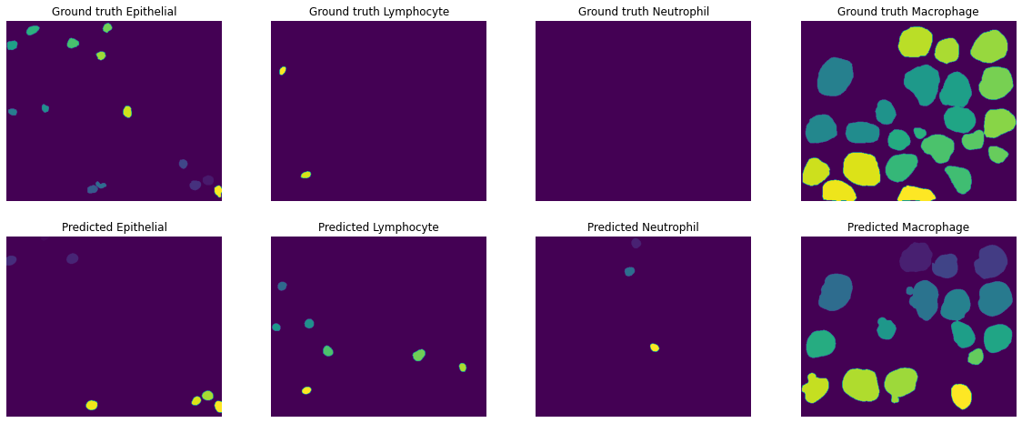
The provided example .mat files illustrating the format chose the "indices following each other" method, so that the indices for a given class will typically only start at 1 for the first class present in the image. The code building the "n-ary masks" from the .xml annotations for the ground truth follow that same rule. In the submission file provided to us by Dr Mahbod, however, the indices are mixed. For the image shown in Figure 8.5, the epithelial indices are for instance [1, 4, 5, 33, 36, 37, 38], and the lymphocyte indices are [11, 16, 17, 23, 25, 28, 32]. We can use that same image to see the effects of this error on the computation of the metric.
The error in the metric computation is stronger when the indices are “misaligned.” In Figure 8.7, the instance labels from the ground truth annotations and the submission file are shown for the same image. In Table 8.2, the results from the computation of the and the number of FP found are reported, using the code used for the challenge and our code with the typo corrected. Apart from the neutrophils, where there was no ground truth object, all other classes are affected by the error in the code. For the macrophages in particular, 9 of the 16 predicted objects are counted as both TP and FP. Notably, the range of the error is somewhat diluted by the nature of the PQ itself. As the PQ multiplies the detection F1-Score with the average of the TP, the error on the F1-Score is less visible.
| Challenge | Corrected | Both | |||||
|---|---|---|---|---|---|---|---|
| Epithelial | 0.379 | 5 | 0.480 | 0.451 | 1 | 0.571 | 0.789 |
| Lymphocyte | 0.298 | 6 | 0.400 | 0.331 | 5 | 0.444 | 0.746 |
| Neutrophil | 0. | 3 | 0. | 0. | 3 | 0. | 0. |
| Macrophage | 0.555 | 9 | 0.667 | 0.683 | 0 | 0.821 | 0.832 |
After our comment article [3], the authors acknowledged this error and recomputed all the scores of the challenge in their reply [18]. Their updated results show that for most teams the difference between the updated PQ and the initial PQ is around 0.04, but that some teams are more strongly affected. Dr Mahbod’s team, for instance, see their initial submission’s score move up from 0.389 to 0.548, gaining three places in the ranking. It is possible that their labelling strategy is the main cause of their poor performance in the original ranking. As we can see in Table 8.3, re-labelling the predicted labels so that they follow each other from class to class considerably lower the effect of the error.
| Labels from submission file | Re-labelled | Corrected code | |
|---|---|---|---|
| With undetected FP error. | 0.536 | 0.566 | 0.596 |
| FP error corrected. | 0.410 | 0.429 | 0.456 |
8.3.2 Undetected false positives
In addition to the error in the computation of the , the challenge code also contains an error in the aggregation of the into the per-image . The way that the code processes a team’s predicted mask is to start from a list of files taken from the ground truth directory. Each of this file will contain the n-ary mask for one class on one image. Iterating through this list, the code then finds a corresponding .mat file in the team’s predictions directory, which had to follow the same structure (PATIENT_ID/PATIENT_ID_IMAGE_ID/Class_label/xxx.mat). The is then computed based on these two n-ary masks and added to an Excel file where the and finally averaged could then be computed.
There is, however, no code provided that checks if there were additional files in the team predictions directory that have no corresponding file in the ground truth directory. In the example that we used above, for instance, there are predicted neutrophils but there are no ground truth neutrophils. As the code is written, the prediction file of the neutrophil class is never opened, and the false positive neutrophils are never counted. The for that image would therefore only be computed based on the of the three other classes, and the fact that three additional false positives were found is ignored. In this case, all three falsely predicted objects were present in another ground truth class, which means that the error is at least counted in the “false negatives” of the other classes. Contrary to the assertion in the author’s reply, however, this is not necessarily always the case: these “false positive” could be made on a region that is not annotated at all, and thus be a “false negative” of the background class, which does not contribute to the metric. In that case, the error would not be counted at all.
Even when the false positives really are all misclassifications of objects of another class, the challenge’s approach would still not work. We can see in Figure 8.7 that some predicted lymphocytes are found in the ground truth of the epithelial class. As there are also some ground truth lymphocytes, those misclassifications are counted both as “epithelial false negatives” and as “lymphocytes false positives,” whereas the same error with the neutrophil class is only counted as “epithelial false negative.”
To avoid this problem, the logical solution would be to set the to 0 when there is a false positive and no ground truth object. As we can see in Table 8.3, this has a considerable effect on the scores. It does seem very harsh to set the to 0 for what may be a single error, which would have a big impact on the and eventually the . This is in large part due to the next problem: the aggregation strategy.
8.3.3 Aggregation strategy
The third big issue with the challenge evaluation is the aggregation strategy. As explained above, the challenge first computes the per-class and per-image, then computes a per-image, and finally computes the average over the 101 images of the test set. Those images, however, are actually small regions extracted from 25 WSI (each one from a different patient). The images, meanwhile, have a very large range of sizes and number of objects. The smallest image only has 2 annotated nuclei, whereas the larger images can have hundreds of them. The published methodology from the challenge organisers is a bit unclear on what they intended to do. In the author’s reply, they clearly state that this was a methodological choice and not an implementation error. The confusion may have stemmed in part from their post-challenge publication, which states that the final is computed from the “[a]rithmetic mean of the 25 ,” and that “[p]articipants submitted a separate output file for each of the 25 test images,” while the pre-challenge preprint often refers to the 101 images as “sub-images.” Regardless of whether the choice of aggregating per-image rather than computing the per-patient (first compiling the TP, FP, FN and IoUs for each “sub-image” of the patient) was intentional or not, it is clearly at the very least a large methodological flaw.
The diversity in image sizes means that errors in small images have a much bigger impact on the overall score as errors in large images. The author’s reply justifies this strategy by the need to compute statistics (in their case, confidence interval on the scores). However, if the samples are the image regions, those that come from the same patient will not be independent. The size diversity also makes the distribution of results much noisier. Even though the number of samples is higher, the statistical analysis is necessarily flawed if the metrics themselves are flawed. A per-patient aggregation still provides enough samples (N=25) for some statistical analysis, with samples that make a lot more sense from a clinical point of view. As we can see in Table 8.4, the errors in aggregation method and with the missed false positives partially “cancel” each other: the correct aggregation method leads to higher PQ overall (as no single errors are penalized too harshly), while adding the previously missed false positives obviously lowers the score, and correcting the computation, which added false positives, increases the score once again.
| Original aggregation method | Corrected aggregation method | |
|---|---|---|
| With undetected FP error. | 0.596 | 0.618 |
| FP error corrected. | 0.456 | 0.563 |
8.3.4 Error in the reporting of the per-class results
A minor issue, which was corrected by the authors in their reply, also appeared in the detailed results published as supplementary materials, where the scores were computed per-organ and per-class. The macrophage and neutrophil classes were inverted in the results. This was simply the result of an “inadvertent column-header swap” [18]. This is very likely given our own analysis, as everywhere in the code the same class order is used with neutrophils before macrophage, but the order is reversed in the supplementary material’s table.
8.3.5 Corrections and scientific publishing
The challenge organisers were contacted and notified of the first error (in the computation of the Detection Quality) in September 2021. They initially replied that the code was correct and, upon receiving evidence that it was not the case, stopped responding. The IEEE Transactions on Medical Imagining editor in chief was contacted in October 2021 and made aware of the problem, and our comment article summarizing our findings was submitted on October 20th, 2021. On February 23rd, 2022, we received notice that our comment article was accepted. It appeared online on the April 2022 issue of the journal, alongside the authors’ reply.
Between October 2021 and April 2022, there was no notice on the original publication that there was any dispute on the validity of the results. The original article is still accessible (and available for purchase) in its original state, with a link to the comment article provided in the “Related Content” tab but no clear indication that the results published inside are incorrect. As not all corrections were accepted and implemented by the authors, the actual results of the challenge are still uncertain at this stage and are likely to remain so.
While it is perfectly normal that editors take the time to make sure that comments and notice of errors on published materials are properly reviewed before issuing a correction, it does not seem right to take no action at all once it is clear that there is at least some credibility to the claims. The choice of not correcting the original article or have a clear notice pointing to the correction, but to publish the comments and authors’ reply separately in another issue of the journal is also strange, as it reduces the trust that a reader can have in currently published results.
8.4 Discussion and recommendations: reproducibility and trust
The terms “reproducibility” and “replicability” are used sometimes interchangeably and with contradicting conventions to refer to two distinct ideas [10]:
The ability to regenerate the results using the original researcher’s code and data.
The ability to arrive at the same scientific findings by an independent group using their own data.
This first definition is crucial in ensuring trust in the published results and is particularly important in the context of digital pathology, deep learning, and challenges. Challenges on complex tasks, as in most digital pathology competitions, often require ad hoc code for the processing of the participants submissions and their evaluation. The opportunity for errors to appear in the implementation of this code is fairly high. There are also many small implementation choices that may influence the results and are not necessarily always reported in the methodology, whether by oversight or by space constraints in the publications.
It is therefore crucial for the source code of the evaluation process to be made available. After publication of the competition results, making the test set “ground truth” annotations available is also necessary to avoid future researchers having to re-create their own train/test split and making improper comparisons of their results with the state-of-the-art. While it obviously creates the possibility of improper management of this dataset by those researchers (i.e. training their model also on the test set to obtain better results), this risk would be best countered by requiring the code of those publications to also be publicly released, rather than by keeping an embargo on the annotations.
While some competitions may prefer to keep an “online leaderboard,” with the possibility for researchers to keep submitting new results that are automatically evaluated, this does not fulfil the requirements for independent reproducibility of the results. To have full reproducibility, the participants submissions and/or their own source code must also be made available.
These may seem like extreme requirements for a competition, but our analysis of the challenges in this thesis shows that the potential for error or misinterpretation is very high. The Seg-PC 2021 challenge, for instance, requires participants to submit segmentation masks for instances of multiple myeloma plasma cells, with labels indicating the pixels that belong to the cytoplasm, and the pixels that are part of the nucleus. The evaluation code, available on the Kaggle platform[^66], shows however that the ground truth and submission masks are binarized so that the “nucleus” and “cytoplasm” labels are merged into a single “cell” label, on which the IoU is computed. The ranking of the challenge therefore does not take into account whether a particular method correctly identifies the nucleus from the cytoplasm. This is a fairly important information for correctly interpreting the results of the challenge, and the fact that the source code is public makes it much more obvious in this case, as the methodology was not clear on that issue.
Mistakes can happen in all parts of the deep learning process in digital pathology pipeline: from the collection and labelling of the data, to the generation of the predictions, the evaluation of those predictions, and the reporting of the results on a website or in a peer-reviewed publication. Transparency on the whole process is key in building trust in the published results, which is undoubtedly necessary before deep learning algorithm can be safely included in clinical practice.
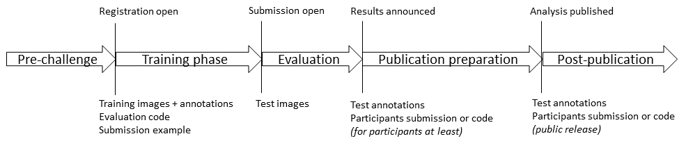
A proposed timeline for the release of the different data necessary to ensure the reproducibility of challenge results is presented in Figure 8.8. As soon as the challenge opens (or before), the images and annotations from the training set should be released, as well as the evaluation code and an example of the expected submission format. This ensures that participants are able to participate in the quality control of the challenge and are able to independently verify that the evaluation process corresponds to the methodology described by the organisers. This also allows participants to give feedback on aspects of the evaluation that the organisers may have overlooked well before the evaluation period, so that the code and methodology can still be adjusted. After the announcement of the results at the end of the evaluation period, the test set annotations and the participants’ submission files (or code) should be made available to at least all challenge participants. In this way, when preparing the post-challenge publication, participants can again independently verify that the evaluation was done correctly and fairly. This can also stimulate challenge participants to contribute interesting insights on the results, thus “crowd-sourcing” the results analysis to a larger pool. Participants can therefore play a more active role in preparing the post-challenge publication, with all the necessary data at their disposal. After publication, all the data should be available to the larger research community, to ensure full transparency and reproducibility.