---- 5.1 Imperfect annotations
------ 5.1.1 Semi-supervised learning from incomplete annotations
------ 5.5.2 Weakly supervised learning from imprecise annotations
------ 5.1.3 Learning from noisy labels
---- 5.2 Datasets and network architectures
------ 5.2.1 Datasets
------ 5.2.2 Baseline networks
---- 5.3 Experiments on the effects of SNOW supervision
------ 5.3.1 Corruption methodology
------ 5.3.2 Experiments and evaluation
------ 5.3.3 Results
---- 5.4 Experiments on learning strategies
------ 5.4.1 Learning strategies
------ 5.4.2 Evaluation procedure
------ 5.4.3 Results
---- 5.5 Comparison with similar experiments
---- 5.6 Impact on evaluation metrics
---- 5.7 Conclusions
5. Deep learning with imperfect annotations
As noted in the 2017 survey of deep learning in medical imaging by Litjens et al. [15], “the main challenge [in medical image analysis] is not the availability of image data itself, but the acquisition of relevant annotations/labelling for these images.” With the increasing availability of whole slide scanners, large datasets of pathology images can now be assembled, but their annotations require highly trained experts and a lot of time [29], [25].
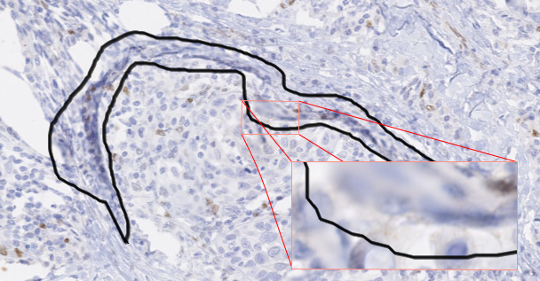
This is particularly the case for segmentation problems, where the “ground truth” is determined at the pixel level. Pixel precise annotations, however, would require a prohibitively large time commitment from the experts, and in many cases would in any case be made impossible by the limitations of the resolution of the image. The exact position of the boundary between regions is often fuzzy and ill-determined in digital pathology datasets, even ignoring the time constraints. As objects of interest can be very numerous and very small, annotations may often not be done at the highest possible available resolution, which means that annotations which seem very precise at the level at which they were made be a lot less accurate at a higher level of magnification (as illustrated in Figure 5.1).
The uncertainty on the accuracy of the annotations can have several causes. As we have already established, there is the inherent uncertainty caused by the acquisition process, with the fuzzy boundaries of the target objects. Another source may be the annotation software or hardware used by the expert. Annotations made with a mouse on a standard computer monitor may be less accurate than annotations made with a stylus on a high-end drawing tablet. The expert may also make mistakes, either in the interpretation of the image or in the manipulation of the annotation tools. A different type of annotation uncertainty comes from the absence of a unique “ground truth”: independent expert annotators, faced with the same image and the same instructions, may produce different annotations.
In this chapter, we will focus on the first type: uncertainties that are caused by imperfections in the annotations. In the next chapter, we will consider uncertainties that come from interobserver variability, or the absence of a singular “ground truth.”
First, we will characterize imperfect annotations using well-known paradigms in machine learning: semi-supervised learning, learning with noisy label, and weakly supervised learning. This will lead us to the concept of “SNOW” supervision (Semi-supervised, NOisy, and/or Weak), that we introduced in [6] and developed in [7]. We will review the state of the art on dealing with the different types of imperfections. We will then present our experiments on the effect of SNOW on segmentation tasks, and on which learning strategies are useful to counteract these effects. Finally, we will examine how our knowledge of these imperfections should affect our evaluation process.
5.1 Imperfect annotations
In the previous chapter, we have defined datasets in the best-case scenario, where each sample is associated to a corresponding ground truth annotation. To describe the different types of imperfections, we need to introduce some notations for the rest of this chapter. is the set of images, and is the set of pixel values in the image . is the set of available annotations, and is the set of true target values that would exist in an ideal dataset.
We define three main types of imperfections, illustrated in Figure 5.2:
![Figure 5.2. Illustration of the three types of imperfection, using as an example an image from the GlaS challenge [22]. From left to right: incomplete (semi-supervised), noisy and imprecise (weak).](./fig/5-2.jpg)
- Incomplete annotations
In incomplete annotations, there is a subset of for which there is no corresponding annotation. This can happen at the pixel level (i.e. within an image , there are some with a corresponding , and some without) or at the image level. Using classical machine learning paradigms, this corresponds to semi-supervised learning. In digital pathology segmentation or detection tasks, it is for instance very common to have expert annotations only for selected focal regions in a WSI. The majority of the WSI, however, may be left unannotated. This can also apply to higher-level tasks such as image classification, where some images may not have expert labels associated to them.
- Imprecise annotations
This corresponds to annotations where the level of details of the annotations is less than that of the target ground truth. Using our notation, this would mean that labels are assigned only for sets of . Practically, this could mean in segmentation tasks that only bounding boxes, or in extreme cases only image-level labels were provided on some or all of the examples, even though the target of the algorithm is to provide a segmentation. This type of imperfection is generally addressed through weakly supervised learning.
- Noisy annotations
With noisy annotations, even when each target ground truth has a corresponding annotation, this annotation may be incorrect. In other words, for each it is possible that . The likelihood of such errors determines the level of noise of the dataset. This type of imperfections can take different forms depending on the type of task. In segmentation or detection tasks, this could correspond to objects that are missed by the annotator. In classification tasks, this could correspond to a wrong label being assigned to the object or image.
Several recent studies have been published in recent years looking at different aspects of imperfect annotations in medical imaging. Karimi et al. [12] experimented on three types of label noise: systematic error by a human annotator, interobserver variability, and label noise generated by an algorithm. Tajbakhsh et al. [27] categorized imperfections into “scarce annotations” (similar to our “incomplete” definition) and “weak annotations” (which include both imprecise and inaccurate annotations). Zhang et al. [33] surveyed techniques for “small sample learning,” which include aspects of incomplete and imprecise annotations. Vădineanu et al. [28] studied annotation errors in cell segmentation, with both inaccurate and imprecise annotations being considered. While this topic has only recently started to be more thoroughly investigated for deep learning and digital pathology, it has been largely covered in classical machine learning through the notions of semi-supervised learning, weakly supervised learning, and noisy labels.
5.1.1 Semi-supervised learning from incomplete annotations
In semi-supervised learning, the dataset can be divided in two subsets: the labelled set , and the unlabelled set where and are the number of labelled and unlabelled instances in the dataset, respectively. It will generally be the case that , as obtaining unlabelled instances is much easier than obtaining annotations.
Zhu and Goldberg [35] describe two main approaches to semi-supervised learning. The first approach is to start from a standard supervised algorithm, and to use the unlabelled data to strengthen the classification from the few labelled data. The second is to start from an unsupervised algorithm, such as clustering, and to use the labelled data to obtain a better clustering (and to label the clusters). The key assumptions made in both approaches are local consistency (i.e. similar samples share the same label) and its counterpart exotic inconsistency (i.e. samples with low similarity are likely to come from different classes) [17]. As noted in Su et al. [26], these assumptions may not always hold for histopathological images, which can have high inter-class similarity and intra-class variation.
An example from classical machine learning applied to digital pathology can be found for instance in Peikari et al. [18]. A “seeded clustering” method is first used to propagate the labels from to and to estimate the density function of the feature space. This density is then used to train a SVM classifier so that it finds the maximum margin boundary region that passes through sparse regions of the feature space.
These ideas have also been applied to deep learning in digital pathology in recent years. Chen et al. [3] use a DCNN to learn features based on sparse labels, then propagate these labels based on affinity in feature space. They apply this method to gland segmentation and tumour region segmentation with promising results based on very few annotations. Shaw et al. [21] propose a “teacher-student chain” based around a ResNet-50 architecture, where is first used to train a teacher model, which predicts “pseudolabels” on . The pseudolabels with a high level of certainty (according to a set threshold) are kept forming a new “supervised” set . is then used to train a “student” model, which is then fine-tuned on . The student then becomes the teacher, and the cycle is repeated. Their method is tested on the NCT-CRC-HE-100K multi-class patch classification dataset [13]. A similar approach is used by Jaiswal et al. [10] for lymph node metastases patch classification on the PatchCamelyon dataset1.
5.5.2 Weakly supervised learning from imprecise annotations
The typical framework for weakly supervised learning (WSL) is Multiple-Instance Learning (MIL). In MIL, instances of the data are grouped into bags , so that labels are only assigned to the bags. Instead of the fully supervised dataset , we therefore have a weakly supervised dataset . The most common application of this framework to visual recognition is to have image-level labels for an object-level task like detection, or a pixel-level task like segmentation. As introduced by Dietterich et al. [1], MIL describes binary problems with a “positive” and a “negative” class, and assumes that any bag that contain at least one positive instance is “positive.”
T. Durand, in his Ph.D. thesis [34] identifies a way of implementing MIL in a deep learning framework. The idea is to use global spatial pooling (for example, max pooling) from a layer that still contains spatial information. With max pooling, the image-level score is therefore the score of the region with the maximum predicted value, which is in line with the principle of MIL that one positive “instance” (in this case: region) is enough to classify the whole bag (in this case: image) as positive. The localization of the detected object can therefore be inferred from the activation of the feature maps. A similar idea is used by methods such as Grad-CAM [20], which uses the activation of the feature maps to highlight the regions of the image that contribute to a class prediction. The main challenges that face WSL algorithms are the difficulty of differentiating strongly co-occurring objects (for instance: boat and water, or chair and table), and of identifying the whole object instead of its most discriminative part (for instance: the face instead of the whole person) [2].
An early application of MIL in digital pathology was proposed by Xu et al. in 2014 [31], in which image-level binary labels (cancer vs non-cancer) are used to obtain pixel-level segmentation and patch-level clustering of distinct cancer types. A deep learning adaptation of MIL was proposed in 2017 by Jia et al. [5], where a DCNN is used to produce pixel-level segmentation at different scales, from which the image-level prediction is determined. The loss function can therefore be computed based on the image-level labels, but the network has to produce a pixel-level prediction as well. Additional area constraints are placed on the segmented regions to penalize unlikely predictions. Chen et al. [3], which we already mentioned for the label propagation in semi-supervised learning, also proposes a WSL method by using superpixels, computed using the SLIC algorithm [14], to propagate points annotations to a larger region.
5.1.3 Learning from noisy labels
Label noise means that, for any annotated label , there is a certain probability that the corresponding ground truth is different. Frénay and Verleysen proposed a taxonomy of label noise [24] that describes three models of noise:
- Noisy completely at random: the occurrence of an error is completely independent from either the true class or the observed data: is constant . In such models, it is furthermore assumed that in a multiclass problem erroneous labels are also uniformly distributed between the other classes.
- Noisy at random: the occurrence of an error depends on the true class but not on the observed data. This means that the noise distribution can be described using a noise transition matrix: .
- Noisy not at random: the occurrence of an error depends on the true class and on the observed data. This model recognizes that, within a class, there will be examples that will be more likely to be mistakenly labelled (for instance, because they are more similar to examples from other classes, or because they are dissimilar to most other examples, meaning that they are in a more sparsely populated region of the input space).
Typical methods outside of deep learning to deal with label noise include data cleaning (i.e. excluding samples that are more likely to be wrong based on, for instance, outliers detection), adapted loss functions, or soft labels reflecting the uncertainty [23]. Frénay and Verleysen categorize three types of methods for handling noisy labels [24]: those that adapt the model selection and design (including loss function and training procedures), those that reduce the noise in the training data, and those that train the classifier and model the noise concurrently.
Karimi et al. [12] review deep learning methods that include some form of noisy label management. The main categories that they identify are: label cleaning and pre-processing; adapted network architectures that include specialized layers that reduce the influence of noisy labels [32], adapted loss functions such as the IMAE loss [30]; data re-weighting that down-weight samples that are more likely to have incorrect labels; adding constraints on data consistency (i.e. samples of the same class should be close in feature space); and adapted training procedures such as co-teaching [8]. In their own experiment on MRI data, Karimi et al. [12] obtain good results with a simple data re-weighting method where data samples with high loss values are ignored, and with a more involved method dubbed “iterative label cleaning,” where a model for detecting noisy labels is updated alongside the main classifier. Using adapted loss functions, meanwhile, did not provide any improvement compared to their baseline network.
5.2 Datasets and network architectures
5.2.1 Datasets
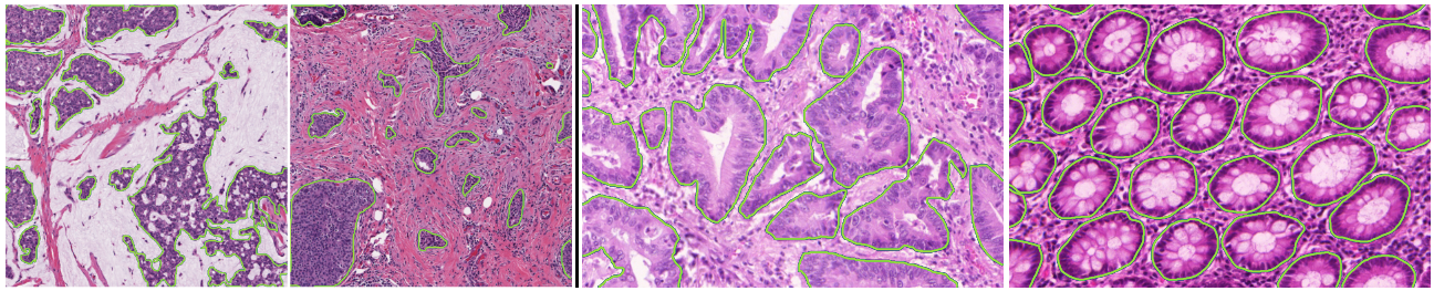
The two datasets used in our experiments are the GlaS challenge dataset [22] and the Epithelium dataset from Janowczyk and Madabhushi [11]. Both contain high quality segmentation annotations of all the target objects in the images. The GlaS dataset targets glands in colorectal tissue (from normal and tumour regions), while the Epithelium dataset separates epithelial from stroma regions in breast cancer tissue. Examples of images and annotations from these datasets are shown in Figure 5.3.
The GlaS dataset has a very high density of foreground objects, with 50% of the pixels in the training set being annotated as positive. The Epithelium dataset, meanwhile, has a slightly lower density with 33% positive pixels in the training set. Our baseline networks are trained using small patches extracted from the larger images of the datasets. For the GlaS dataset, we used 256x256px patches, and around 95% of the extracted patches contain at least some part of a gland, and would therefore be considered “positive” patches in a MIL framework. For the Epithelium dataset, 128x128px patches were used, with around 87% “positive” patches.
The GlaS dataset is used for the experiments on the effects of SNOW, while both datasets are used for the experiments on the learning strategies. Additional information on the datasets can be found in Annex A.
5.2.2 Baseline networks
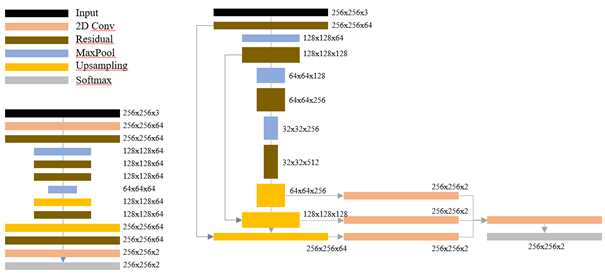
Three networks were used for our experiments: ShortRes, U-Net and PAN. They all follow a classic segmentation macro-architecture with an encoder and a decoder. The “ShortRes” network uses short-skip connections similar to ResNet [9] in the encoder and in the decoder, and has around 500k parameters. U-Net is directly adapted from Ronneberger et al.’s version [19], with long-skip connections between the encoder and the decoder and Dropout layers. It has around 30M parameters. The third network, which we called “Perfectly Adequate Network” (PAN), uses both short and long-skip connections, and combines the outputs from different layers to produce the final segmentation using multi-scale predictions. It has around 10M parameters. These 3 architectures allow us to study networks with a priori different learning capacities and to measure their respective resistance to different types and/or levels of supervision defects. In all the networks, the Leaky ReLU [16] activate function are used in the convolutions and transposed convolutions. A schematic representation of the ShortRes and PAN architectures is shown in Figure 5.4.
In all our experiments, the same basic data augmentation scheme is applied to the training sets that are then used by all networks, left as is (baseline) or combined with one of the learning strategies described below. We modify each mini-batch on-the-fly before presenting it to the network, using the following methods:
Random horizontal and/or vertical flip.
Random uniform noise on each of the three RGB channels (maximum value is 10% of maximum image intensity).
Random global illumination changes on each of the three RGB channels (maximum value of ± 5% of maximum image intensity).
5.3 Experiments on the effects of SNOW supervision
To assess the effects of SNOW supervision on deep neural networks, we introduced “corrupted annotations” to clean datasets. These corrupted annotations were generated to simulate different levels of supervision and annotation effort. In this section, we will detail the methodology for the corruption, and show the effect on the three baseline networks. In the next section, we will look at how different learning strategies can help to deal with the effects of SNOW supervision. The results presented here were originally reported in our SNOW publications [6], [7], with some additional assessment.
5.3.1 Corruption methodology
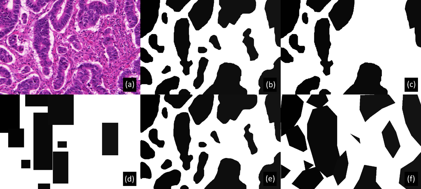
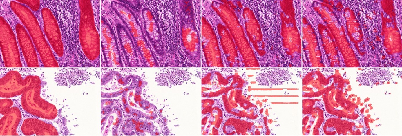
As illustrated in Figure 5.5, random corruptions are introduced in the training set annotations of both datasets mimicking imperfections commonly encountered in real-world datasets. The test set with correct annotations is kept to evaluate the impact of these imperfections on DL performance. Pseudo-code for the procedure used to generate the corrupted annotations is given in Table 5.1.
| Corruption of the annotations | |
|---|---|
| Let be the noise level. | |
| Let be the standard deviation of the radius of the erosion/dilation disk. | |
| Let be the simplification factor for the contour. | |
| Let be the original dataset, with images and corresponding annotations | |
| Output: the corrupted dataset | |
| 1 | For each : |
| 2 | For each annotated object in and corresponding object in : |
| 3 | Draw from uniform distribution |
| 4 | If : remove from |
| 5 | Else: |
| 6 | Draw from normal distribution |
| 7 | If |
| 8 | Else: |
| 9 | Compute all points in contour of |
| 10 | Sample points in (regular sampling) to create contour |
| 11 | Compute filled polygon raster of from |
Because creating pixel-perfect annotations is very time-consuming, experts may choose to annotate faster by drawing simplified outlines. They may also have a tendency to follow “inner contours" (underestimating the area of the object) or”outer contours" (overestimating the area). We generate deformed dataset annotations in a two-step process. First, the annotated objects are eroded or dilated by a disk whose radius is randomly drawn from a normal zero-centered distribution, a negative radius being interpreted as erosion and a positive radius as dilation. The standard deviation () of this distribution enables us to adjust the level of deformation. The second step consists in simplifying the contour of each object, as follows. The contour pixels are identified and only a fraction of them, determined by a simplification factor , are kept to create a polygonal approximation of the original contour. The median number of points in the object contours in the original annotations is 358. We introduce low deformations using and (median of 36 remaining points per contour), medium deformations using and (median of 9 remaining points per contour), and high deformations (see Figure 5.5) using and (median of 5 remaining points per contour).
In addition to deformed annotations, we also simulate the case where the expert chooses a faster supervision process using only bounding boxes to identify objects of interest. In this case, we replace each annotation by the smallest bounding box which includes the entire object.
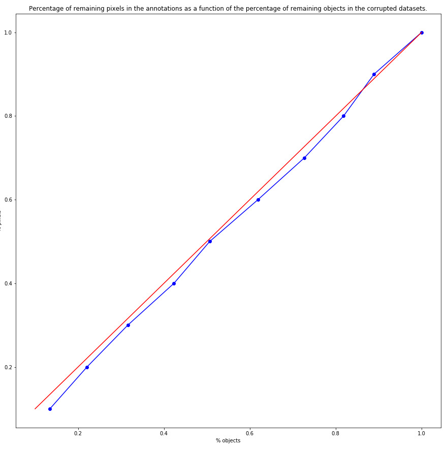
Experts who annotate a large dataset may miss objects of interest. We create “noisy datasets" by randomly removing the annotations of a certain percentage of objects. A corrupted dataset with”50% of noise" is therefore defined as a dataset where 50% of the objects of interest are relabelled as background. As there is some variation in the size of the objects, we verified that the percentage of pixels removed from the annotations ranged linearly with the percentage of omitted objects, as shown in Figure 5.6.
Different imperfections are also combined: noise with deformations and noise with bounding boxes, resulting in different "SNOW datasets", as illustrated in Figure 5.5.
5.3.2 Experiments and evaluation
The following experiments were performed on the GlaS dataset:
Compare the corrupted annotations to the ground truth annotations. This estimates the performance of a model that perfectly matches the imperfect annotations.
Measure the performance of the three networks based on different levels of noise, erosion/dilation radii and simplification factors.
The DSC was used as a general-purpose binary segmentation metric in these experiments, as the goal was not to focus on any particular use case but to look at the overall effect of SNOW imperfections on the performances of the algorithms. Each network was trained once on each of the randomly corrupted training dataset, then evaluated based on the original annotations of the test set.
5.3.3 Results
The results of the first experiment are presented in Table 5.2. A low amount of deformation is associated with a 4% loss in the DSC. This indicates that when a pixel-perfect segmentation is difficult to define (for instance with objects with fuzzy or debatable boundaries), results based on typical segmentation metrics should be interpreted carefully. In such a situation, a difference of a few percent between two algorithms could thus be considered as irrelevant.
| Dataset | DSC (Corrupted vs Original, training set) | DSC (ShortRes vs Original, test set) |
|---|---|---|
| Original (GlaS) | 1.000 | 0.841 |
| 10% Noise | 0.931 | - |
| 50% Noise | 0.589 | 0.231 |
| Low deformation () | 0.960 | - |
| Medium deformation () | 0.917 | - |
| High deformation () | 0.830 | - |
| Bounding boxes | 0.836 | 0.724 |
| 50% Noise + High deformations | 0.455 | 0.212 |
| 50% Noise + Bounding boxes | 0.557 | 0.511 |
:Table 5.2. DSC of different corrupted datasets compared to the original ground truth annotations (in the training set), alongside the DSC for the ShortRes trained on the corrupted annotations (measured on the original test set).
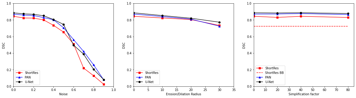
Figure 5.7 shows the effects of increasing noise levels introduced in the supervision of the GlaS training set on the performance of the 3 baseline DCNNs. Despite their differences in terms of size and architecture, the three networks behave very similarly, with some robustness up to 30% of noisy labels. However, a clear decrease in performance is observed from 40% or 50% of supervision noise. The effects of annotation erosion or dilatation are much less drastic, and polygonal approximations seem to have no significant effects in the range of considered in these tests. For ShortRes, the performance on the “bounding boxes” dataset, which can be seen as an extreme form of polygonal simplification, are about the same as the effects of large erosion/dilations. The three networks behave in a very similar way with regard to these types of annotation corruption. It should be noted that the the variability of the results due to the randomness of the corruption process is not taken into account in those results. However, the overall trends identified in the results are unlikely to be affected by this randomness. Uncertainty in the measured results may increase for the largest values of the corruption parameters, but these values correspond to such a large performance drop on the three networks that the effect is very unlikely to be a random anomaly.
Somewhat surprisingly, as shown in Table 5.2, the ShortRes network trained on the combined “50% noise + bounding boxes” corruptions actually performs better than the network trained on the 50% noise with no deformation dataset. This is likely to be a result of the very high object density of this particular dataset. As the bounding boxes cover more tissue area, they may give the networks a bias in favour of the positive pixel class, which helps them get a better score on the uncorrupted test set: as we have shown in Chapter 4, overlap-based metrics such as the IoU or the DSC are biased in favour of results that overestimate the segmented region.
5.4 Experiments on learning strategies
The next set of experiments we performed aimed at assessing the performance of different learning strategies on the corrupted datasets. Given the very similar behaviours observed above for the three baseline networks with respect to SNOW supervision, only the ShortRes network is used in the first experiments on the GlaS datasets to investigate the effects of different learning strategies. This allows us to draw the first lessons that we then confirm on the Epithelium dataset using the ShortRes and PAN networks, knowing that original versions of both datasets are similar in terms of the quality and nature of the annotations.
5.4.1 Learning strategies
For the following strategies, we consider two subsets of the training data. The positively annotated regions () corresponds to all pixels which are within a 20px margin of the bounding box of an annotated object in the dataset. The negatively annotated regions () corresponds to all remaining pixels. Practically, we first compute the bounding boxes of all objects annotated in the training set and extend their boundaries by 20px in all directions. When sampling patches, a patch is considered “in ” if it intersects with at least one pixel of these extended bounding boxes, and “in ” otherwise.
5.4.1.1 Only Positive (OnlyP)
In this approach, only input patches in are used for training the model.
5.4.1.2 Semi-supervised learning (SSL)
A two-step approach (see Figure 5.8) is used for the semi-supervised strategy and is based on the fact that all our networks follow the classic encoder-decoder segmentation architecture described in section 1.5.2.
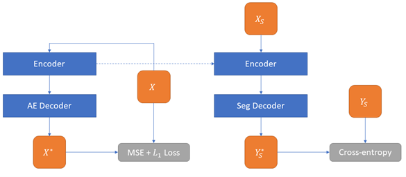
First, an auto-encoder (AE) is trained on the entire dataset by replacing the original decoder (with a segmentation output) by a shorter decoder with a reconstruction output. The Mean Square Error loss function between the network output and the input image is used to train the auto-encoder, with an L1 regularization loss on the network weights to encourage sparsity.
The second step consists of replacing the decoder part of the AE by the decoder of the segmentation network, and then training the whole network on the supervised dataset. The encoder part of the network is therefore first trained to detect features as an auto-encoder, and then fine-tuned on the segmentation task, while the decoder of the final network is trained only for segmentation. In the experiments on the SNOW datasets reported below, we test two variants of the semi-supervised strategy depending on the supervised data on which the network is fine-tuned: either the full supervised (and corrupted) dataset, or only patches from . This latter version will be referred to as “SSL-OnlyP” in the result tables.
5.4.1.3 Generated Annotations (GA)
The “Only Positive" strategy may tend to overestimate the likelihood of the objects of interest, especially in cases where they have a fairly low prior (such as in our artefact dataset, used in Chapter 6). We propose a slightly different, original approach based on a two-step method detailed as follows (with pseudo-code in Table 5.3). First, we train an annotation generator network with patches sampled from (i.e. using the”Only Positive" strategy). This annotation generator is then used to reinforce the learning of the final segmentation network, which will be trained on the whole dataset using the following procedure. If the patch is in , the original annotations are used as supervision. If it is in , it randomly chooses between using the original (empty) annotations or the output of the annotation generator as supervision. The probability of each choice should depend on the object prior. As the original datasets are quite strongly biased towards the presence of objects of interest, we use a probability of either 75% (GA75) or 100% (GA100) of using the annotation generator output.
| Generated annotations strategy | |
|---|---|
| Let be the generator model | |
| Let be the segmentation model | |
| Let be all the image patches and corresponding annotations in the positive regions, and for the negative regions. | |
| 1 | Train using the patches sampled from |
| 2 | Train : procedure for each minibatch |
| 3 | Initialize as the current minibatch |
| 4 | Sample patch |
| 5 | If : |
| 6 | Append to |
| 7 | Else: |
| 8 | Draw (uniform distribution) |
| 9 | If : |
| 10 | Append to |
| 11 | Else |
| 12 | Compute |
| 13 | Append to |
| 14 | Repeat until desired batch size |
This strategy can be seen as a version of semi-supervised learning because the regions without annotations are sometimes treated as “unsupervised" rather than with a”background" label. But it is also based on label noise estimation. The assumption that positive regions are more likely to have correct annotations results in a highly asymmetric noise matrix, with , where is the true class and the class provided by the imperfect supervision. The Generated Annotations strategy includes this information by treating positive annotations as correct for training and negative annotations as uncertain.
5.4.1.4 Label augmentation (LA)
Knowing that labels could be imperfect, especially around the borders, we create slightly modified versions of the supervision via morphological erosion or dilatation (with a 5 pixels radius disk) of the objects of interest that are randomly presented during learning. Following a purpose similar to that of classical data augmentation, this strategy aims at making networks robust to annotation modifications.
5.4.1.5 Patch-level annotation strategies
As mentioned above, typical weak strategies rely on patch-level annotations. However, such strategies are not appropriate for the datasets described in section 5.2.1, because these sets include very few examples of negative patches (5% for GlaS and 13% for Epithelium). This means that with original or noiseless datasets, "weak" networks would see almost only positive examples, whereas with noisy data sets, they would see either correct positive examples or incorrect negative examples. In either case, they will not be able to learn. Therefore, these strategies were not used in our experiments.
5.4.2 Evaluation procedure
The networks are trained with patches randomly drawn from the training set images. The patch size is determined for each dataset by preliminary testing on the baseline network, with the goal of finding the smallest possible patch size on which the network can learn. 256x256 pixels patches were selected for the GlaS dataset and 128x128 pixels patches for the Epithelium dataset. To evaluate the results on the test set, images are split in regular overlapping tiles, with 50% overlap between two successive tiles. For each tile, the networks produce a probability map. As most pixels (except those close to the borders) are seen as part of multiple tiles, the maximum probability value for the "positive" class is assigned as the final output. A mask is then produced using a 0.5 threshold applied to this final output. It should be noted that contrary to what is usual in image segmentation, no further post-processing is applied on the results. This aims to avoid contaminating the experiences by external factors but with the consequence of somewhat penalizing our baseline networks compared to what is reported in the literature.
We initially used the DSC as a general-purpose metric for both publicly available datasets and their corrupted versions, as the objective of this experiment is not to solve a particular digital pathology task, but to compare the effects of the learning strategies on segmentation accuracy. The DSC is computed for each image of the test set. To determine significant differences between the strategies, in terms of performance achieved with a given training set, the DSC obtained on the same test image are compared by means of the Friedman test and the Nemenyi post-hoc test, as described in Chapter 4. The DSC, however, is (like the IoU) asymmetrical in its treatment of over-estimation vs under-estimation of the segmented region. In a dataset where the proportion of positive tissue is so large, the DSC of a method that mostly predict positive pixels everywhere will be much better than that of a method that is more conservative in its predictions. We therefore also compute the per-pixel MCC to take the “true negatives” into account in the evaluation, thus treating the segmentation task as a per-pixel binary classification task. While the MCC is not a commonly used segmentation metric, its symmetrical properties are nonetheless useful in gathering insights on the behaviour of the different learning strategies and can capture information that are not easily detected with the DSC.
On the GlaS dataset, a "statistical score" is also computed to highlight the actual differences in performance between the tested strategies. For each corrupted dataset and for each pairwise strategy comparison, if the difference between the two strategies is judged significant by the post-hoc test (), a positive point is assigned to the best learning strategy and a negative point to the other. The statistical score is computed by summing those points for each learning strategy. The best learning strategies so determined are then applied on the Epithelium dataset.
5.4.3 Results
5.4.3.1 Results on the GlaS dataset
The average DSC and MCC on the GlaS test set of the learning strategies are reported in Table 5.4, alongside the statistical score. The first notable thing is that all learning strategies outperform the baseline method on most corrupted training sets. Using the DSC, it appears that the three most effective learning strategies overall are the “Only Positive” and the two “Generated Annotations” methods. The “Only Positive” results, however, are far less impressive when looking at the MCC, particularly on the “50% Noise + High deformations” (NoisyHD) dataset. This is due to a strong bias towards positive predictions on that particular dataset. From the MCC results, the two “Generated Annotations” methods appear to outperform the others, with the SSL-OnlyP method as the only other method that, on average, outperforms most others.
| DSC | Original | Noisy | BB | NoisyBB | NoisyHD | Stat. score |
|---|---|---|---|---|---|---|
| Baseline | 0.841 | 0.231 | 0.724 | 0.511 | 0.212 | -22 |
| OnlyP | 0.836 | 0.768 | 0.730 | 0.697 | 0.660 | 10 |
| SSL | 0.831 | 0.467 | 0.756 | 0.522 | 0.207 | -11 |
| SSL-OnlyP | 0.819 | 0.729 | 0.740 | 0.730 | 0.428 | 5 |
| GA100 | 0.837 | 0.764 | 0.755 | 0.700 | 0.621 | 12 |
| GA75 | 0.843 | 0.736 | 0.754 | 0.695 | 0.608 | 10 |
| LA | 0.837 | 0.575 | 0.761 | 0.631 | 0.449 | -4 |
| MCC | Original | Noisy | BB | NoisyBB | NoisyHD | Stat. score |
| Baseline | 0.683 | 0.231 | 0.355 | 0.328 | 0.200 | -18 |
| OnlyP | 0.668 | 0.577 | 0.409 | 0.450 | 0.012 | -1 |
| SSL | 0.664 | 0.372 | 0.474 | 0.347 | 0.186 | -6 |
| SSL-OnlyP | 0.647 | 0.537 | 0.413 | 0.487 | 0.070 | 5 |
| GA100 | 0.664 | 0.588 | 0.455 | 0.413 | 0.438 | 11 |
| GA75 | 0.687 | 0.573 | 0.453 | 0.410 | 0.433 | 11 |
| LA | 0.674 | 0.450 | 0.488 | 0.337 | 0.322 | -2 |
The per-dataset results show, however, that the learning strategies have different strengths and weaknesses when it comes to the types of imperfection in the annotations. The SSL-OnlyP strategy, for instance, significantly outperforms all others when trained on the “50% Noise + Bounding boxes” (NoisyBB) set, where the OnlyP method also performs relatively well. Both perform very poorly, however, when trained on the NoisyHD set. The SSL and LA methods, meanwhile, have the worse performances overall (outside of the baseline), yet they still perform well when trained on the “Bounding boxes” (BB) set (although all methods have very similar results when using those annotations).
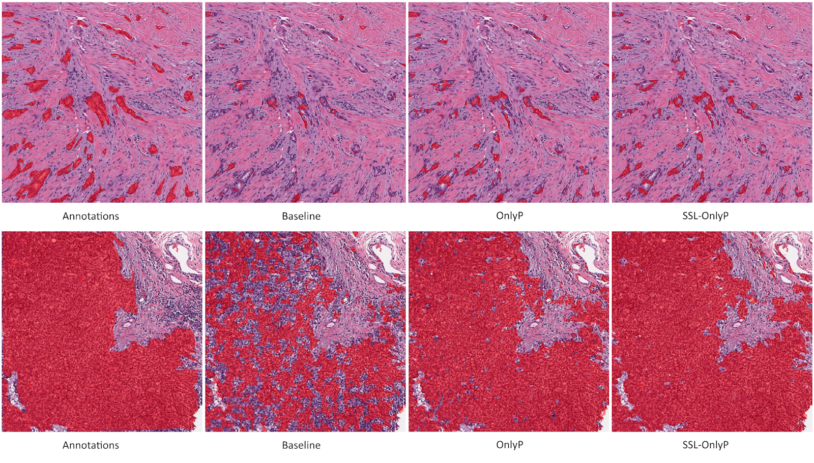
Results of the “50% Noise” (Noisy) training on some images from the test set are shown in Figure 5.9. The baseline network severely underestimates the target regions. The OnlyP strategy recovers a lot of the performance but has large regions of false positives. The GA100 offers a form of compromise between the two, and generally has the best results overall. The raw results could be considerably improved in all cases with some basic post-processing (such as morphology operations), but these raw results make the effects of the learning strategies more visible.
5.4.3.2 Results on the Epithelium dataset
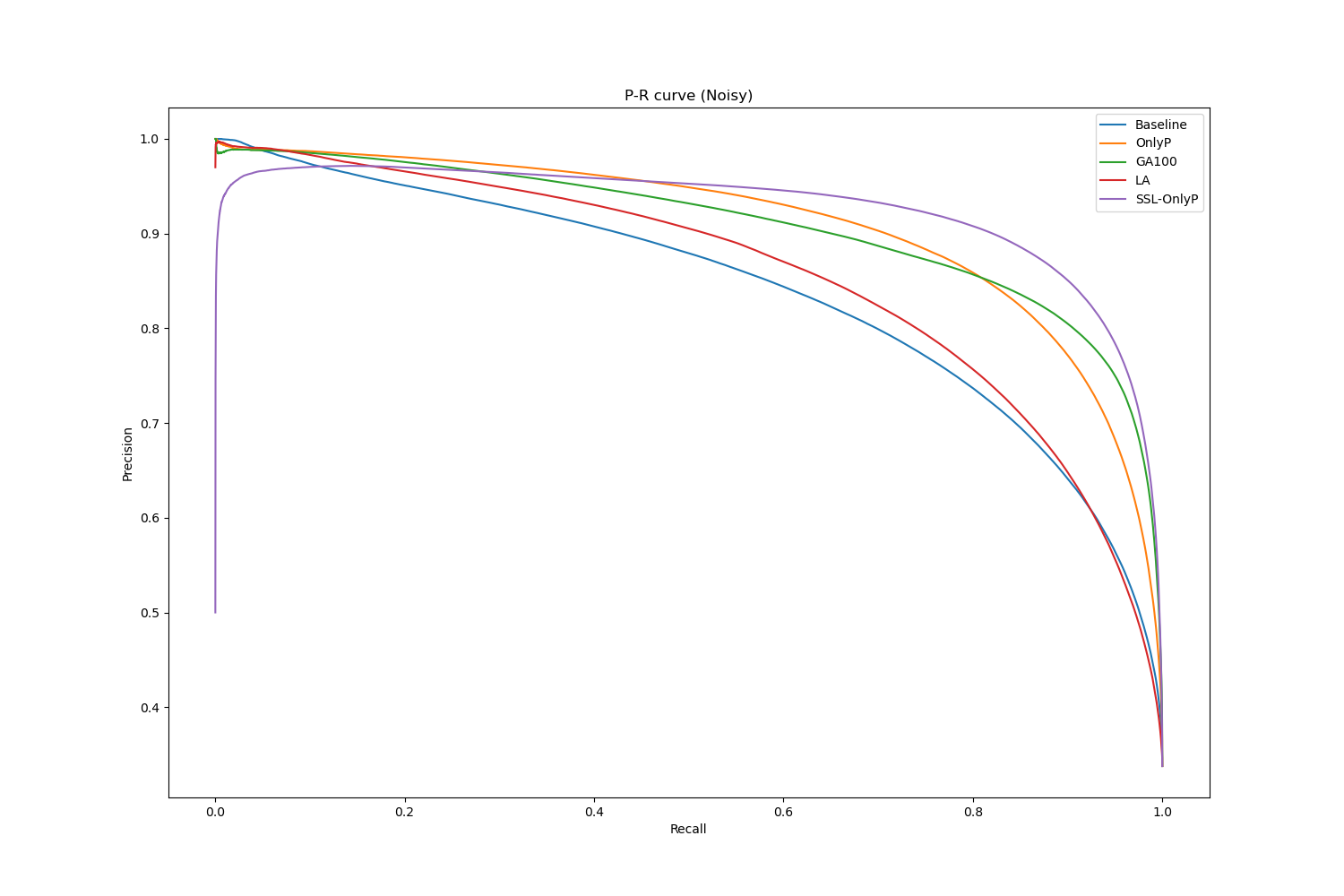
The average DSC and MCC on the Epithelium dataset of the different learning strategies are reported in Table 5.5. To get some additional perspective on the results, we also report the Average Precision (AP), which is the area under the precision-recall curve. A single AP is computed on all test images at once, so no statistical test was done for that metric.
| DSC | Original | Noisy | Deformed | |
|---|---|---|---|---|
| Shortres | Baseline | 0.853 | 0.545 | 0.811 |
| OnlyP | 0.848 | 0.730 | 0.808 | |
| GA100 | 0.848 | 0.671 | 0.809 | |
| LA | 0.837 | 0.577 | 0.808 | |
| SSL-OnlyP | 0.853 | 0.788 | 0.816 | |
| PAN | Baseline | 0.860 | 0.639 | 0.828 |
| OnlyP | 0.857 | 0.762 | 0.826 | |
| GA100 | 0.861 | 0.681 | 0.827 | |
| LA | 0.858 | 0.648 | 0.814 | |
| SSL-OnlyP | 0.853 | 0.768 | 0.788 | |
| MCC | Original | Noisy | Deformed | |
| Shortres | Baseline | 0.781 | 0.466 | 0.717 |
| OnlyP | 0.767 | 0.646 | 0.714 | |
| GA100 | 0.770 | 0.595 | 0.717 | |
| LA | 0.777 | 0.489 | 0.733 | |
| SSL-OnlyP | 0.778 | 0.718 | 0.747 | |
| PAN | Baseline | 0.786 | 0.559 | 0.746 |
| OnlyP | 0.783 | 0.685 | 0.746 | |
| GA100 | 0.788 | 0.606 | 0.744 | |
| LA | 0.785 | 0.572 | 0.731 | |
| SSL-OnlyP | 0.774 | 0.684 | 0.740 | |
| AP | Original | Noisy | Deformed | |
| Shortres | Baseline | 0.952 | 0.845 | 0.929 |
| OnlyP | 0.952 | 0.913 | 0.921 | |
| GA100 | 0.951 | 0.912 | 0.923 | |
| LA | 0.948 | 0.861 | 0.932 | |
| SSL-OnlyP | 0.955 | 0.931 | 0.948 | |
| PAN | Baseline | 0.953 | 0.886 | 0.938 |
| OnlyP | 0.953 | 0.924 | 0.934 | |
| GA100 | 0.954 | 0.919 | 0.936 | |
| LA | 0.957 | 0.888 | 0.933 | |
| SSL-OnlyP | 0.957 | 0.924 | 0.943 |
Those results confirm that the baseline networks are robust even to large deformations of their annotations. They also confirm that, for the noisy annotations, strategies that focus the training on the areas with “positive” pixels (which are more likely to be correctly annotated) manage to recover well even from a dataset with 50% of annotations removed. Even though the difference is not statistically significant according to the Nemenyi post-hoc, the Semi-Supervised method does seem to perform slightly better with the ShortRes network. The Label Augmentation method, meanwhile, does not outperform the baseline even on the deformed dataset.
An interesting insight from computing the AP is that the baseline appears more robust than when looking at the single-threshold metrics, even on the noisy labels. This indicates that, while a lot of positive tissue is missed using the standard 0.5 threshold at the output, the predicted value is still generally higher in positive tissue than in negative tissue. The Precision-Recall curve on the noisy labels dataset, shown in Figure 5.10, provides some additional information on the behaviour of the strategies. The SSL-OnlyP method has a better AP than the other strategies, but it also has an “inverted U” shape that indicates that it has some very high confidence false positive predictions.
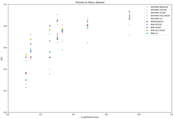
The results on the Epithelium dataset also illustrate how important the distribution of the dataset is to the results. As Figure 5.11 shows, the image where the different models have the worst performance according to the DSC and MCC metrics is an image with relatively few objects of interest. Conversely, the image where the models perform best is one which is nearly entirely covered in “positive” (epithelial) tissue. This is confirmed in Figure 5.12, which plots the relationship between the ratio of epithelial tissue in an image and the DSC of the networks and learning strategies. Images with sparse epithelial tissue are clearly associated with lower values for the DSC and MCC.
5.5 Comparison with similar experiments
Similar experiments to our 2019 [6] and 2020 [7] publications have since then been made by Karimi et al. [12] and by Vadineanu et al. [28].
Karimi et al. introduced increasing levels of realistic deformations on foetal brain annotations in diffusion weighted MR images. They show that their baseline network (with a U-Net like architecture) is fairly robust to levels of deformation similar to our experiments, and that the results only start to fall when the DSC of the deformed set compared to the original annotations becomes lower than around 0.8 (our “high deformation” dataset had a DSC of 0.830). They compare two learning strategies: using an adapted loss function, and an “iterative label update” method which is similar in principle to our “GA” method. The latter has better performances in general for most noise levels, although the adapted loss function is slightly better for extreme levels of deformations. However, no statistical analysis was provided and the results in general are relatively close even with the baseline, so it is difficult to draw strong conclusions from their results.
Vadineanu et al., meanwhile, introduced label noise and deformations in a very similar fashion to our experiments (with the addition of “inclusion” errors, i.e. “negative” objects labelled as “positive”) for cell segmentation in immunofluorescence images, and for epithelial nuclei segmentation using the MoNuSAC 2020 dataset. They only studied the effects of the noise on baseline networks but did not introduce additional learning strategies. Their results show that the networks are relatively robust to up to 30% of label noise with, like in our experiments, a big fall in performance starting at 40-50% noise. They show a stronger sensitivity of their networks to deformations. However, their target objects are very small and the metric used is the DSC, which means that even small deviations from the annotated “ground truth” are harshly penalized, as evidenced in Chapter 4, section 4.4.6.
5.6 Impact on evaluation metrics
While we have focused in this chapter on the impact of SNOW annotations when training a DCNN, we should not neglect the impact on evaluation metrics. Even when experts are instructed to take more time on the test set annotations, or when senior experts are more involved in the validation of these annotations, there will always remain some level of imprecision and noise (even neglecting interobserver variability). This impact is, by its very nature, extremely difficult to objectively assess. It should, however, not be neglected. As an example, Cruz-Roa et al. [4] note in their 2014 publication on invasive ductal carcinoma detection that “[a] closer examination of the qualitative segmentation results suggests that some misclassifications (both FP and FN errors) are a result of imperfect manual annotation.”
A first possibility for evaluating an algorithm using SNOW annotations is to use a very small subset of the test set so that several experts can agree on the best possible annotations for that subset, then to compare those annotations to the corresponding test set “ground truth.” This can provide a lower boundary to the range of differences in metrics between algorithms that cannot reasonably be considered to be true differences in performances. For instance, if the DSC between the “optimal annotations” and the “test set annotations” in a segmentation problem is 0.98, then a difference lower than 0.02 in the DSC should always be considered as an ex aequo, before any statistical testing even needs to be applied.
The other approach is to accept the uncertainty on the value of the metric, and to instead look at the SNOW annotations in the context of the discussion of the results. This can include having an expert look at randomly selected errors from the evaluated algorithms and assessing the likelihood of the algorithm being correct. One possibility for a fair assessment would be to show examples of regions where the “ground truth” and the “prediction” are different and ask the expert to choose the best of the two (ideally in a blind setting). While it would generally be impractical to apply this kind of analysis to all errors and all algorithms (particularly in the context of a challenge where tens or hundreds of methods are being compared), performing it even on a small subset of the data would at least provide an idea of the difference in performance that needs to be observer between the algorithms to be reasonably certain that one outperforms the other.
5.7 Conclusions
Deep learning models are trained and evaluated on a “ground truth,” which is assumed to be exact. Practically, this is however not the case. Imperfections are unavoidable in any dataset, but they are particularly important in digital pathology. Segmentation tasks are the most difficult to properly annotate, as they require pixel-precise supervision on objects which are often very small, and which can have irregular, fuzzy boundaries. It is also impractical to annotate entire WSI for detection or segmentation: supervision will therefore always be limited to a set of regions of interest.
There has been a lot of work on how to manage those imperfections for training deep neural networks, and to best leverage the annotations that are available despite their imperfections. For segmentation, it is clear that deep neural networks are relatively robust to strong deformations, and to limited amounts of noise. This suggests that the best annotation strategy is to be exhaustive within a region of interest in the identification of the objects, without necessarily being precise about the exact boundaries. Using polygonal approximations rather than trying to pixel-precise, for instance, would generally be sufficient and considerably speed up the annotation process. The best learning strategies, meanwhile, harness the full unsupervised dataset to determine the best feature space, and focus the learning of the discriminative part of the network on the well annotated regions. Re-labelling unannotated regions (or mislabelled regions in the case of multi-class problems) may be useful as well, particularly when the annotated subset if small.
The question of how to deal with imperfect annotations for the evaluation of the algorithms has been less explored. All evaluation metrics assume the existence of a perfect ground truth, so that predictions can be categorised as “correct” or “incorrect.” It is generally difficult to really include the uncertainty due to imperfections to this computation, as evaluating the level of imperfection would require, in turn, a perfect “ground truth” for comparison. To get out of this circular problem without ignoring it, evaluation processes should include a review by experts of the errors made by the algorithms to assess the proportion of these errors that may be attributed to mistakes in the annotations themselves rather than in the predicted labels.
Imprecise, noisy and incomplete annotations are unavoidable in real-life applications. Ensuring that deep neural networks are capable of handling SNOW annotations in their learning process is crucial to their clinical application. Furthermore, recognizing these imperfections in the evaluation procedure is necessary to avoid rewarding algorithms that reproduce the imperfections and penalizing algorithms that may be as good or better at the clinical task despite being less similar to the available “ground truth.”