---- 7.1 Pathology
------ 7.1.1 Tumour grading
------ 7.1.2 Mitosis detection
------ 7.1.3 Gleason scoring
---- 7.2 Computer vision
------ 7.2.1 Comparing automated methods with pathologists
------ 7.2.2 Consensus methods for ground truth generation in challenges
------ 7.2.3 Influence on training deep learning models
---- 7.3 Evaluation from multiple experts
---- 7.4 Insights from the Gleason 2019 challenge
------ 7.4.1 Effect of the Gleason score computation method
------ 7.4.2 Impact of consensus method
------ 7.4.3 Visualizing expert and consensus method agreement
---- 7.5 Discussion
7. Interobserver variability
A key characteristic of digital pathology tasks is the absence of a 100% reliable ground truth. Pathology is a domain where inter-expert disagreement is typically high. There have been many studies on the importance of interobserver variability for clinical practice, and many computer vision publications note and often measure in some way this disagreement for the particular dataset that they are working on, it is rarely, if ever, taken into account into the evaluation process. In this chapter, we will review the importance of interobserver variability in pathology tasks in general (section 7.1), then more particularly in the context of image analysis challenges and other image analysis publications (section 7.2). We will particularly look at how the “ground truth” of the dataset is determined to train and evaluate algorithms, and how researchers’ knowledge about inter-expert disagreement is incorporated into the process.
After these analyses of the state-of-the-art, we will also take a closer look in section 7.4 at a specific digital pathology challenge: Gleason 2019. This challenge is the only image segmentation challenge in digital pathology to date that released individual expert annotations instead of a “consensus” annotation on their dataset, making it a very useful resource when exploring the effects of inter-expert agreement. Our analyses and experiments on the Gleason 2019 dataset in particular were presented at the SIPAIM 2021 conference and published in SPIE [17].
7.1 Pathology
7.1.1 Tumour grading
Inter-expert or interobserver agreement is a long-studies topic in pathology. Cancer grading often relies on a combination of criteria which can be highly subjective, such as the shape irregularity. Interobserver variability is an important factor in assessing the usefulness of cancer grading systems [8]. Indeed, a grading system where the criteria are too subjective and have a high degree of interobserver variability will necessarily be less trustworthy, and more dependent on the level of experience of the pathologist. The 1991 study establishing the Nottingham grading system for breast cancer [12], for instance, clearly states that their modification to the earlier “Bloom & Richardson” method aimed “to introduce greater objectivity,” and they measure their success in part by the fact that “tumours […] graded independently by two experienced histopathologists obtain[ed] over 90% agreement on first assessment.” They also note that “[r]eproducibility between different centres is more difficult to achieve.”
Inter-expert agreement in cancer grading is generally measured as the “rate of agreement” ( in Table 7.1), which is simply the percentage of cases where the two experts assigned the same grade, or with Cohen’s kappa [7] (see Chapter 4, section 4.1.3). Cohen’s kappa is an extremely popular agreement metric in medical studies (despite some important known weaknesses [10] discussed in section 4.3.2). While varies between 0 (no agreement) and 1 (perfect agreement), Cohen’s kappa varies between -1 (complete disagreement) and 1 (perfect agreement), with 0 meaning that the agreement is equal to that expected from random chance.
| Reference | Description of the experiment | Main findings |
|---|---|---|
| Hernandez, 1983 [22] | Two pathologists from different institutions asked for histologic type (5 possibilities) and histologic grade (4 possibilities) of 68 ovarian tumours from 34 patients. | for histologic type, for histologic grade (.) |
| Gilchrist, 1985 [19] | Eleven surgical pathologists studied microscopic sections from 45 masectomy specimens of node positive breast cancer patients. Asked for cell types (2) and nuclear grades (3). | pairwise for cell type (). for nuclear grades () |
| Robbins, 1995 [37] | Consensus of 3 pathologists in an institution compared to consensus of 2 in another on 50 cases of breast cancer in B5 and BFS fixed tissue. Asked for cancer grade, tubule formation, nuclear size/pleomorphism and mitotic count (3 categories each). | on nuclear grade (, , ). on mitotic grade1 (, , ) |
| Özdamar, 1996 [33] | Two pathologists asked to grade prostate cancer using the WHO grading system (4 categories) and the Gleason scores (9 categories) in 96 specimens. | (WHO), (Gleason) |
| McLean, 1997 [29] | Three urology pathologists asked to grade prostate cancer using the Gleason scores in 71 specimens. | Using all Gleason scores (5-9): , , , . Regrouped in 2 categories2: , 3. |
| Allsbrook, 2001 [1], [2] | 41 general pathologists and 10 urologic pathologists asked to grade prostate cancer using the Gleason score in 38-46 cases. The study measured the agreement between urologic pathologists, and between general pathologists and the consensus of the urologic pathologists. | , 4 pairwise agreement. General pathologists (measured against the consensus of urologic pathologists): |
| Meyer, 2005 [30] | Seven pathologists asked to grade breast cancer in five trials. Also reports several earlier studies. | on tumour grade (. on mitotic grade (). |
| Malpica, 2007 [28] | Nine pathologists (incl. 2 non-specialists) asked for grading of 80 cases of ovarian serous carcinoma (in two rounds to also measure intraobserver agreement) | Pairwise |
| Paech, 2011 [36] | Meta-analysis of six studies on interobserver variability in lung cancer grading. | , |
| Davidson, 2019 [9] | 208 pathologists interpret 1 of 4 breast cancer biopsy sets including 5 or 6 invasive carcinomas, then interpret the same set 9 months later in a randomized order (for intraobserver agreement), either using a glass side or a WSI. | on Nottingham grade. on Mitotic count. |
| Bulten, 2020 [5] | Two pathologists asked to grade prostate cancer TMA cores using Epstein groups. | , , |
As detailed in Chapter 4, section 4.1.3.2, Cohen’s kappa can take different forms, depending on whether the categories used by the observers are ordered on not, and if ordered depending on how much “large” errors should be penalized. The “unweighted” kappa ( henceforth) penalizes all errors equivalently, while the linear () and quadratic () kappa values penalize errors that are “smaller” less harshly, so that in situations where most errors are between neighbouring categories.
Interobserver agreement does not just depend on the task, but also on the specificities of the dataset, the instructions given to the observers, the conditions of the test, etc. This makes a direct comparison of interobserver agreement between studies difficult, even when looking at the same underlying pathology task. For instance, in a meta-analysis of lung cancer interobserver variability studies, Paech et al. [36] find that even after reanalysing the results to ensure that all studies measure the same classes, rates of agreement vary between 77% and 94% (with the ranging between 0.48 and 0.88). Such large variations in results can be also seen for other cancer types, such as ovarian cancer [22], [28] or breast cancer [19]–[30].
The reason for interobserver disagreement is often found either in subjective criteria, or in criteria that are difficult for humans to perceive objectively, such as relative proportions. As noted in Hernandez et al. when discussing their results [22], “Although observers A and B agreed as to what cell types were present, they did not always agree as to which cell type was more prevalent and representative of the tumor.”
Meyer et al. also note regarding breast cancer grading that “[t]his and other studies show that while disagreements of one step (grade 1 vs grade 2, grade 2 vs grade 3) have been common, discrepancies of more than one grade seldom occur” [30]. It is interesting to note that, while this is obviously a very important criterion in assessing interobserver variability, many studies appear to use the as their agreement metric, even though it is completely invariant to the degree of the disagreements.
7.1.2 Mitosis detection
Mitotic count is an important factor in tumour grading, particularly in the Nottingham system for breast cancer grading. Most of the studies on breast cancer grading therefore also report the agreement on mitotic grade. The mitotic grade is a grouping of the mitotic count in three categories, using thresholds that depend on the field area of the microscope [12]. Meyer et al. [30] report the results from several studies between 1982 and 2000, finding values ranging from 0.36 to 0.70 for mitotic grade.
It is noteworthy that mitosis detection, as it is generally conceived as a computer vision task, will typically be evaluated on a per-mitosis basis, whereas the clinical relevance is mostly found in the categorized mitotic grades. The evaluation of computer vision algorithms should therefore at the very least discuss the potential clinical impact of their performance in addition to the classical image analysis metrics.
7.1.3 Gleason scoring
Several grading systems have been proposed for prostate cancer over the years, but by the mid to late 1990s the Gleason system had become the most widely used [29]. Part of the reason for its widespread adoption (and for later revisions) is its higher correlation with patient outcome compared to competing systems [43], another cited factor has been its relatively higher inter- and intraobserver agreement, making it more reliable and less dependent on a particular pathologist. As Özdamar et al. [33] state, “[t]hose items with poor agreement cannot be regarded as reliable indicators and cannot be used for making a decision,” and only a system with similar intra- and interobserver variability “may be safely used by different pathologists.”
The high subjectivity of the Gleason pattern grading, however, is made apparent in a 1997 study by McLean et al. [29], where they find that, without a prior “consensus meeting” between the pathologists to agree on the precise criteria they would use to assess those patterns, they obtained relatively poor rates of agreements (between 0.18 and 0.37 on three possible pairings of pathologists, with ranging from 0.15 to 0.29).
Two large studies by Allsbrook et al. in 2001 have been largely cited since then, measuring interobserver agreement between 10 urologic pathologists [1], then measuring the performance of 41 general pathologists against the consensus of the urologic pathologists [2]. They found markedly higher agreement than in the McLean study, with pairwise ranging between 0.48 and 0.84. General pathologists had an even wider range of results, with 2/41 achieving almost perfect agreement with the “consensus” of urologic pathologists, yet 7/41 fairing barely better than random chance, showing the importance of specialised training and experience on such a complex problem.
A major update to the Gleason system was made first in 2005, then in 2014 at the International Society of Urological Pathology Conference [13], leading to the “Epstein grouping” system. Some changes were made over the year in the exact definition of each pattern, but the Epstein system brings some major changes in the final categories. This major update largely simplifies the interpretation of the results (5 groups instead of 10 scores), and was validated as better correlated with patient outcome [14].
The effect on interobserver agreement, however, is less clear. A 2016 study by Ozkan et al. [34] found very little difference in agreement between the Gleason score () and the Epstein groups ()5. The importance of which “kappa” is used is clearly shown if we try to compare the 2016 study with the recent 2020 study by Bulten et al. [5], which reports a for two pathologists on 245 Tissue Micro Arrays samples for Epstein grouping. This seems like a much higher agreement than the 2016 study, but that interpretation depends on which kappa they actually used, as recomputing the kappa from Bulten et al. gives us and , meaning that the agreement is either vastly improved, slightly improved or even slightly worse. As Bulten et al. provide the confusion matrix in their supplementary materials, it is easy to recompute the different values as needed, but the Ozkan et al. study gives little details on how they came to their numbers.
7.2 Computer vision
7.2.1 Comparing automated methods with pathologists
Interobserver variability has been a known problem for a long time in digital pathology. In fact, the introduction of computer vision algorithms to the digital pathology pipeline has often been justified in part by the need to provide more objective, quantitative assessments to reduce this interobserver (and intra-observer) variability in diagnosis [20]. Interobserver variability generally affects computer vision pipelines (and more particularly machine learning algorithms) in two aspects: in the generation of the ground truth (often through a consensus mechanism), and in the evaluation. Very often, for the evaluation, interobserver variability is only considered as a way to compare the performance of algorithms to the performance of pathologists, both evaluated against the “consensus ground truth.”
This type of comparison, however, may be difficult to do fairly. As an example, Bauer et al. [4] compare the performances on a benign/malignant cancer classification task of a ResNet to a classical “handcrafted features” pipeline and to inter-pathologist accuracy. The inter-pathologist accuracy, however, is computed as the proportion of cells which receive the same label from two pathologists (in this case, 1272/1633, or 78%). Meanwhile, the performances of the algorithms are computed based on the 1272 cells where the pathologists were in agreement. This can obviously introduce a large bias, as the cases where the experts are in disagreement are more likely to be more difficult to correctly classify. In the same publication, a more meaningful comparison between the algorithms and the pathologists is also proposed, with both being tested on follow-up survival data.
A different approach is proposed in Turkki et al. [38] to evaluate an automated method for the quantification of tumour-infiltrating immune cells in breast cancer samples stained with H&E. The accuracy is first computed based on a collegial supervision by a group of experts aided by additional IHC images. Then, the results on another set of images are compared to two pathologists separately, and the pathologists are similarly compared with each other.
Malon et al. [27] studied inter-pathologists agreement for mitosis detection. To include an automated method in their comparison, they used the majority vote from three pathologists as a ground truth, and then evaluated each pathologist and the automated method against this ground truth. While this is certainly less biased than removing the contentious cases, it still poses a potential bias problem, as the pathologists in this case are evaluated on a ground truth that they participated in. Indeed, while the algorithms in this case has to agree with 2 of the 3 pathologists for a prediction to be counted as correct, a pathologist only has to agree with one of their two colleagues. This weakness was noted by the authors. One of the effects of this methodology was that it gave a large advantage to one of the pathologists in particular: as the other two were very often in disagreement, this pathologist typically acted as the “tie-breaker” and was therefore largely responsible for the determination of the “consensus.”
A much stronger comparison (which also require significantly more effort and the involvement of more experts) is performed in Bulten et al. [5] for Gleason grading. The ground truth was determined by three pathologists specialised in urological pathology, first independently, then collegially for cases with disagreements. Fifteen additional pathologists with varying levels of experience (including two pathologists in training) and a deep learning algorithm were compared to the consensus. The automated method obtained a better quadratic kappa than the median of the pathologists, outperforming 10 out of 15.
Several deep learning competitions have evaluated interobserver variability in some way. In the AMIDA 2013 mitosis detection challenge [39], the ground truth was initially determined independently by two pathologists, with two additional pathologists reviewing the cases with a disagreement. In the challenge results, they observed that “many of the false positives produced by the top performing methods closely resemble mitotic figures,” and subsequently performed a “re-annotation” of the false positives by two of the pathologists (one from the “first pass,” one from the “reviewers”). About 30% of the false positives from the top method were re-annotated as true positives. The ground truth test dataset was also re-annotated, with only 71% of the objects originally annotated as “mitosis” being relabelled as such. Clearly, such large uncertainty on the real “ground truth” label has the potential to influence the results of a challenge. The BACH 2018 challenge [3] created the “ground truth” with two pathologists which had access to information outside of the H&E images (such as IHC or other regions of tissue), and three other pathologists were tested while being given only the same information as the competing algorithms. A large panel of “external” pathologists was also used in the Camelyon 2016 challenge [11] for metastatic region segmentation in lymph nodes. The Gleason 2019 challenge will be more thoroughly discussed in section 7.4 below.
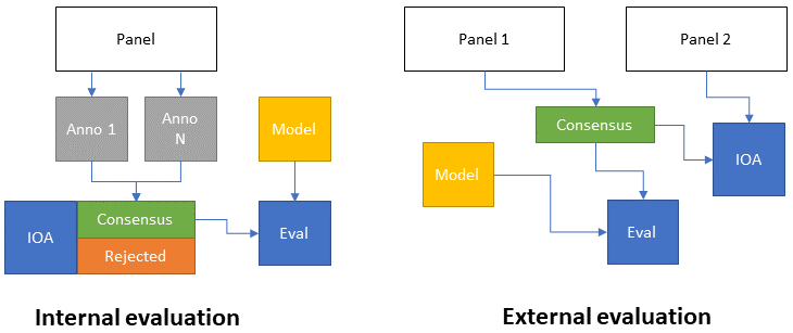
In general, we can therefore see two main approaches to the evaluation of interobserver agreement as a means of providing a comparison to algorithmic performances (as illustrated in Figure 7.1). In internal evaluation, the expert panel creates the dataset by first annotating it separately, then creating a consensus. At the same time, the interobserver variability is computed based on the individual annotations. In some cases, parts of the dataset where no consensus can be reached may be rejected, and the consensus data is used to evaluate the model. In external evaluation, an independent panel of experts is used for the evaluation of interobserver agreement. The main advantage of this approach is that it puts the evaluation of the experts on a “fair” ground with the model. Indeed, for the creation of the consensus dataset, experts can often use more information than what’s available to the model (as the goal is to have the best possible annotations). This fairness comes at the cost of requiring additional experts.
7.2.2 Consensus methods for ground truth generation in challenges
Even when the interobserver variability is not explicitly computed or reported, its existence always means that challenge organizers have to choose how to address it to create the “ground truth” annotations of their dataset.
In our study of segmentation challenges in digital pathology [16], a diversity of strategies was identified for the generation of “ground truth” annotations from multiple experts. The simple solution of using a single expert as ground truth was used by the PR in HIMA 2010, GlaS 2015 and ACDC@LungHP 2019 challenges, with the latter using a second expert to assess interobserver variability.
Several challenges use students (in pathology or in engineering) as their main source of supervision, under the supervision of an expert pathologist reviewing their work. This was the case for the Segmentation of Nuclei in Images challenges of 2017 and 2018 (no information was found for the earlier editions of the challenge), as well as for the MoNuSeg and MoNuSAC challenges.
The Seg-PC challenge in 2021 relied on a single expert for identifying nuclei of interests, then on an automated segmentation method which provided a noisy supervision [18], at least for the training set. It is unclear whether the same process was applied for the test set used for the final evaluation, as that information is not present in the publicly available documents of the challenge.
When using multiple experts, the processes vary and are sometimes left unclear. BACH and PAIP 2019 used one expert to make detailed annotations, and one to check or revise them. DigestPath 2019 and the 2020 and 2021 editions of PAIP all mention "pathologists" involved in the annotation process, but do not give details on how they interacted and came to a consensus. Gleason 2019 used six experts who annotated the images independently. A consensus ground truth was automatically generated from their annotation maps using the STAPLE algorithm [40]. BCSS, NuCLS and WSSS4LUAD used a larger cohort of experts and non-expert with varying degrees of experience, with more experienced experts reviewing the annotation of least experienced annotators until a consensus annotation was produced.
Conic 2022, meanwhile, uses an automated method to produce the initial segmentation, with pathologists reviewing and refining the results.
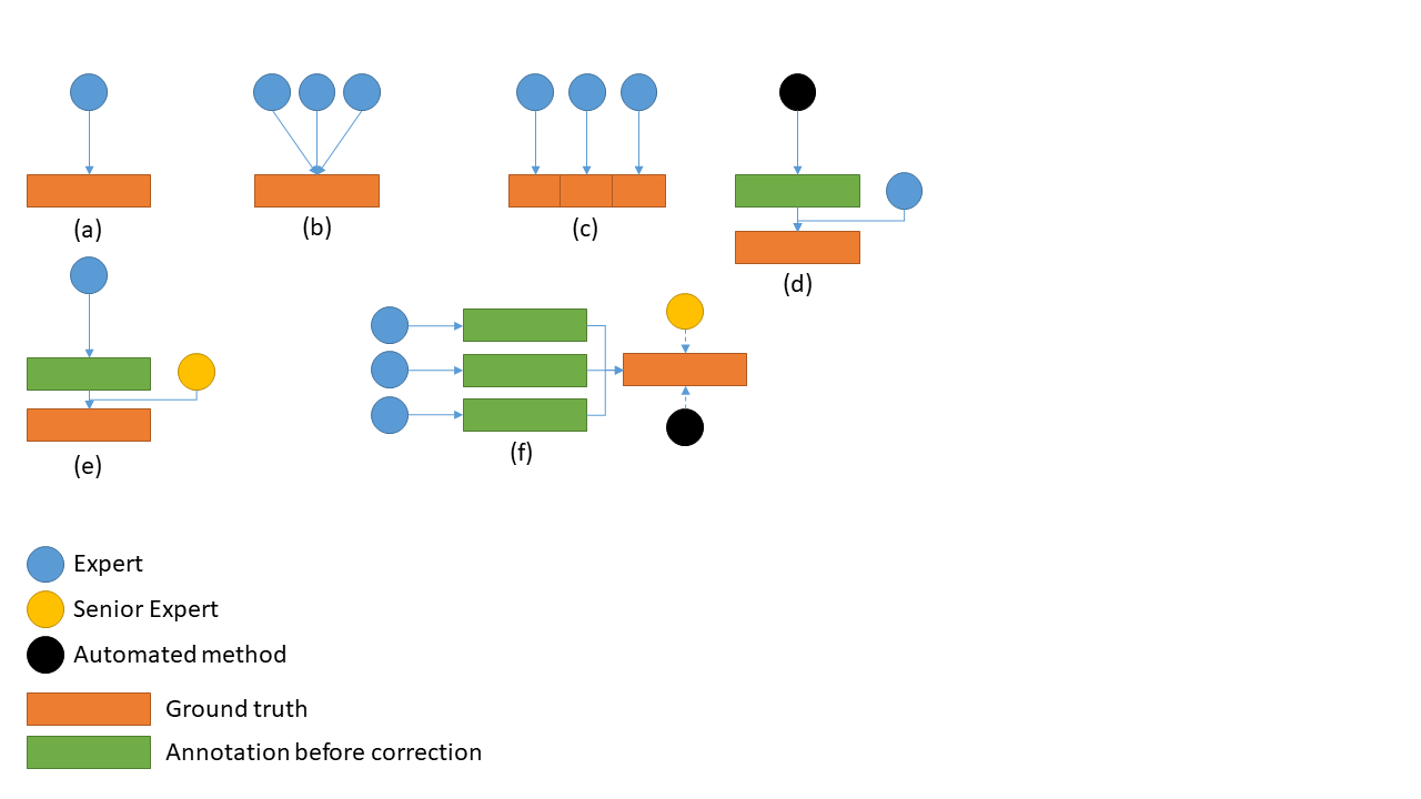
In general, we can identify the following common strategies, illustrated in Figure 7.2:
A single expert being considered as ground truth. In this case, the interobserver variability is unknown or needs to be evaluated separately (having another expert which has no impact on the ground truth produce their own annotations).
Multiple experts working collegially (either working on all cases together, or discussing the cases where there is a disagreement). The interobserver variability is also unknown in this case, as there is no “individual annotations” being produced.
Multiple experts working independently on subsets of the data. The big advantage of this approach is that it is easier to get more data without overworking a single expert. The dataset will also naturally include the diversity in biases and habits of individual experts. There may however be some induced biases if, for instance, some experts are over-represented in the test set.
Automated method refined by expert(s). In this case, it is very easy to quickly get a lot of “noisy” data (using the best algorithms from the current state-of-the-art), with the expert only needed to provide corrections when needed. The resulting annotations may however remain noisy, particularly in segmentation tasks, as the limits of what an expert would consider an acceptable annotation may vary.
Expert with senior review. In this approach, the original annotations are provided by junior experts (one or several working on subsets of the data), and a senior expert checks their annotations. Some insight on the interobserver variability may in this case be extracted from the number of corrections that the senior expert had to make.
Multiple experts producing individual annotations. This approach makes it easy to evaluate the interobserver variability at the same time as the ground truth annotations are generated. Producing those ground truth annotations, however, requires the additional step of “merging” the individual annotations. This can either be done by an automated method (such as majority voting, or the previously mentioned STAPLE algorithm), or with the help of a senior expert which resolves conflicts.
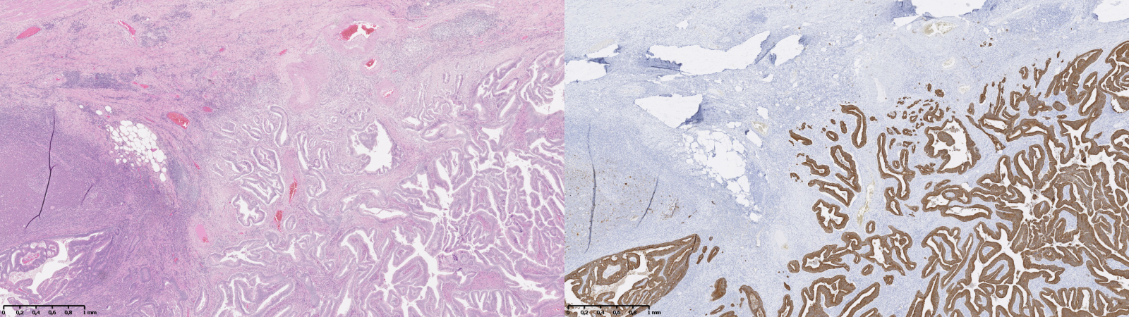
An additional strategy, which bypasses the need for a “consensus,” is to generate the supervision based on additional data. This could come from available information on patient outcome, or from using data from IHC as a supervision for an adjacent H&E-stained slide. The latter approach is used for instance in Turkki et al. [38], where consecutive slides were stained with H&E and the anti-CD45 antibody. The CD45 expression was then used to annotate the H&E slide with “immune cell-rich” and “immune cell-poor” regions. An example of such technique is illustrated in Figure 7.3 using images from our “Artefact” dataset, enabling the identification of epithelial cells (using anti-pan-cytokeratin IHC). The difficulty of such technique is that it requires a correct registration of the IHC image onto the H&E image, as there will always be some deformations, potential tissue damage, different artefacts, etc., between the two. This registration task was the target of the ANHIR challenge in 20196.
7.2.3 Influence on training deep learning models
Just as there are many different approaches to creating a “consensus” ground truth from annotations by multiple experts, several options are available for training deep learning models with these annotations. In most of the ground truth generation strategies, only the consensus annotations set is available in the end, leaving no choice but to train the models based on this “ground truth.” Interobserver variability, in that case, has to be considered as “noisy labels,” as in the previous chapter. When annotations from multiple experts are available, however, more options are available.
In digital pathology, the Gleason 2019 dataset is the only publicly available segmentation dataset to have released those individual annotations. The team from the University of British Columbia that produced the dataset tested several strategies in publications made before the challenge [31], [32], [25]. In a first study [31], a “probabilistic approach,” based on a method by Raykar et al. [21], in which the classifier is trained simultaneously to the “consensus label” and the annotators’ accuracy using an Expectation Maximization algorithm. In another study [25], pixel-wise majority voting is used as the ground truth label. The results are then compared with the same algorithm trained and tested using ground truth labels created with the STAPLE algorithm. They report results that are marginally better (but “very close”) with the STAPLE than the majority vote. In a third publication [32], they compare training on a single expert (and testing on each expert separately) with training and testing on the majority vote. They show that, unsurprisingly, the algorithm performs better when tested on the same pathologist as it was trained on. They also obtain better results using the majority vote labels. However, they do not test using individual annotations from all experts versus using the majority vote labels. Lastly, Karimi et al. [24] compared training on single pathologists, the majority vote labels, and the STAPLE labels, all on a test set ground truth computed with the STAPLE algorithm. Results with majority vote and STAPLE were similar (and better then a single pathologist). They also tested using the separate annotations from three pathologists for training, and the STAPLE consensus of the three others for testing. While these results are not directly comparable (since the ground truth labels are not the same as in the other experiments), they point to similar performances than the STAPLE and majority vote training.
Post-challenge publications from other teams of researchers using the publicly available dataset have also used different strategies. Khani et al. [26] and Jin et al. [23] use the STAPLE labels for training and testing. Ciga et al. [6] and Yang et al. [42] both choose to only use the annotations from a single expert. Zhang et al. [44] merge the annotations to create a per-pixel “grade probability” map (so that if, for instance, three experts predict grade 3 and three experts predict grade 4, the pixel will be associated with a probability vector with p=0.5 for the grade 3 and 4 labels). Xiao et al. [41] use all individual annotations with a custom loss function that give different weights to each expert and each pixel in the images, and additionally weight the pixels based on their “roughness” in the image (defined as the absolute difference between the image before and after a Gaussian filter). They do not specify which “ground truth” they use for their test set, although their illustrations are consistent with either a STAPLE consensus or a majority vote.
In his 2021 Master Thesis at the LISA laboratory [45], Alain Zheng studied the effect of training a deep neural network either on all six separate expert annotation sets, or on the STAPLE consensus, with the test set ground truth always being set to the STAPLE consensus. The results from this Master Thesis show that better predictive performances on the image-level Epstein groups (which are more clinically relevant than the per-pixel predictions) were obtained by the network trained on the separate annotation sets, but that the difference is only significant (according to a McNemar test) if it is combined with a filter that only take into account the pixels where the highest class probability and the second-highest class probability verify .
7.3 Evaluation from multiple experts
While many different strategies are used to generate the ground truth and to use the multi-expert annotations for training, the evaluation of the algorithms is always done on a single reference “ground truth,” typically the result of a consensus process. It is however not necessarily the only way to use annotations from multiple experts when they are available. In this section, we study possible alternatives that may provide better insights on the performances of the evaluated method.
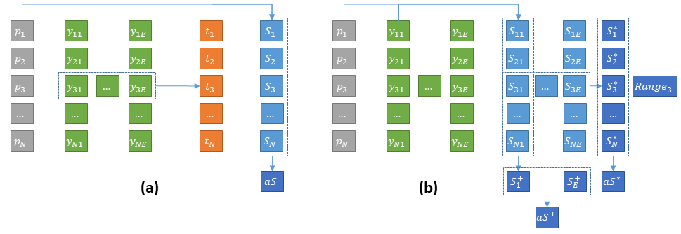
In a multi-expert dataset, each image will be associated with a set of annotations with the number of experts who annotated that particular image (this number may vary between images, as not all experts will necessarily annotate all images). The typical process for using these annotations is to first apply a consensus mechanism to obtain a reference ground truth , where the “consensus” function may be a mathematical process (such as the STAPLE algorithm or the majority vote) or a human process (such as a discussion between the experts to resolve the issue, or a decision by a senior expert). Then, the score per image of a prediction is computed using a metric as:
Statistics based on these scores per image can then be computed, such as the average score on the images, which is usually the “summary statistic” from which algorithms being compared are ranked:
Another approach, however, is to compute the scores independently for each expert annotation, so as to obtain a “per-image, per-expert” score :
Several options are then available. The “consensus” score can be replaced by the average of the per-expert scores :
Which can then be used similarly to , for instance to compute the average score on the dataset:
With this approach, another set of information can give some interesting insights on the algorithm’s behaviour: the degree to which the scores are different depending on which expert provides the annotation. For instance, the per-image standard deviation, or more realistically the range (as there will generally not be many experts per image):
To fully explore the multi-expert aspect of the annotations, however, another strategy is to compare the summary statistics on the dataset per-expert directly, without first computing a per-image average. In that case, a “per-expert” average score can for instance be computed:
If all experts annotated all images (so that is constant), a single average performance can be obtained as:
Otherwise, the per-expert scores should really be considered as separate measures.
Approaching the evaluation from a multi-expert perspective can allow us to make a distinction between algorithms whose errors (relative to the consensus) tend to follow the biases of some of the experts in the dataset, from algorithms whose errors are due to other factors. As the error becomes a set of dissimilarities to different experts, it also becomes possible to use alternative methods to visualize the results, such as the Multi-Dimensional Scaling (MDS) that we previously used to look at the dissimilarity between metrics. In a multi-expert evaluation setup, MDS can be used to visualize at the same time the interobserver variability (how dissimilar the experts are to each other) and the performance of the algorithm (how dissimilar the algorithm is to each of the experts).
7.4 Insights from the Gleason 2019 challenge
In our 2021 SIPAIM publication [17], we further explored the Gleason 2019 dataset and the impact of multi-expert annotations. In this section, we present those results, with some improvements to make our results more relevant to the clinical perspective.
The Gleason 2019 dataset uses “Tissue Microarray” (TMA) slide, which contain many small tissue samples (the “cores”) assembled in a grid pattern on a single slide [35]. In the dataset, individual cores are extracted from those slides and presented as separate images.
Using the publicly available training set of 244 cores, we studied several aspects:
How are inter-expert agreement and agreement to the consensus affected by the Gleason score computation method on each image.
How these agreement levels are affected by the consensus method.
How the comparison between an algorithm and the experts against the consensus may be affected by the participation of the experts in the consensus.
What insights may be gained from a visualisation method such as MDS.
Another aspect that was explored in this publication was the presence of clear mistakes in the annotation maps. This will be left for the next chapter on quality control.
7.4.1 Effect of the Gleason score computation method
The first step in the Gleason grading system is to identify the “Gleason patterns” that are present in the image (see Figure 7.5). The patterns are graded from 1 to 5. The annotations in the Gleason 2019 dataset are segmented glandular regions with their associated Gleason pattern. According to the challenge definition, “[t]he final Gleason score is reported as the sum of the most prominent and second most prominent patterns; e.g., a tissue with the most prominent pattern of Gleason grade of 4 and the second most prominent pattern of Gleason grade of 3 will have a Gleason score of 4+3”7 (if a single pattern is present, the value is doubled, e.g. 4+4). This appears to follow the 2005 ISUP guidelines [15], where the final score is therefore on a scale from 2 to 10. These guidelines were revised at the 2014 ISUP conference [13]. According to these new guidelines, Gleason pattern 1 and 2 are removed. The first group (after “benign” tumours) is therefore constituted by tumours where only pattern 3 is present (3+3 = 6 in the Gleason system). The two next groups are defined are “3+4” (predominant pattern 3 with some pattern 4 present), “4+3” (predominant pattern 4 with some pattern 3), which were previously merged as “score 7.” Finally, we have a “score 8” group and a “score 9-10” group. The scores are thus replaced by “groups” (hereafter “Epstein groups”):
Group 1 = Gleason scores <= 6
Group 2 = Gleason patterns 3+4
Group 3 = Gleason patterns 4+3
Group 4 = Gleason score 8
Group 5 = Gleason score > 8
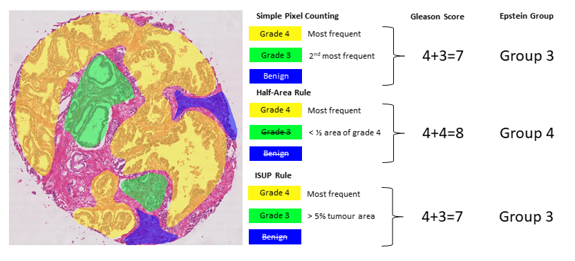
Identifying what counts as “predominant patterns” is not trivial either. For instance, the 2005 guidelines specify that “in the setting of high-grade cancer one should ignore lower-grade patterns if they occupy less than 5% of the area of the tumor” [15, p. 1236]. However, higher-grade patterns should be considered even if they occupy a very small area. This, however, may not necessarily be adapted to automated methods of identifying the Gleason patterns, as it is more likely to have “noisy” results with very small pockets of badly identified patterns influencing the results.
In our analysis, we look at the inter-expert agreement measured by the unweighted and quadratic weighted Cohen’s kappa () for all inter-expert agreements using the Gleason scores (ranging between 2-10) and the Epstein groups (ranging from 1-5). Two rules were tested to identify the two “predominant patterns.” First, a simple pixel counting (SP) rule consists in identifying and summing the two most frequent grades in terms of pixels, except if only one grade is present which is then doubled (e.g. a single grade 4 gives a score of 4+4). In our SIPAIM publication, we also defined a “half-area” rule, according to which the second most frequent grade is considered only if the area with this grade is at least half of the area occupied by the first most frequent grade. This latter rule aimed to give more weight to the majority grade and to avoid possible small “contaminations” due to segmentation errors. However, this rule is too aggressive at removing “smaller” regions compared to what pathologists would typically do (particularly in the presence of small regions of high-grade patterns). We therefore replace this rule here to follow the ISUP guidelines more closely and consider the secondary pattern either if it has a higher grade than the primary pattern, or if it has a smaller grade and occupies at least 5% of the annotated tumour regions. Our SIPAIM publication also used the “grade 1” pattern annotation in the score and group computations (i.e. a core with predominant grade 4 and some grade 1 would lead to a score a 5 and to Epstein group 1). However, the label “1” in the annotations corresponds to benign tissue, so only grades 3 to 5 should be considered. For these reasons, the tables presented here have different values than those presented in the original publication [17]. The different scoring methods are illustrated in Figure 7.5.
Our experiment (see Table 7.2) shows to what extent the results vary depending on the scoring method. On average, the unweighted kappa shows moderate (0.4-0.6) agreement between experts, whereas the quadratic weighted kappa shows substantial (0.6-0.8) agreement, indicating that most of the disagreement happens between scores or groups that are close from each other. The individual head-to-head comparisons (see ranges) using the unweighted kappa vary from moderate (0.2-0.4) to substantial (0.6-0.8), with a perfect (1.) agreement between experts 2 and 6 in the case of the Epstein groups. However, these two experts have very few annotation maps in common and their head-to-head comparison only concerns 4 maps. The quadratic kappa again shows superior values, with several experts having “almost perfect agreement” (0.8-1.).
| G-SP | G-ISUP | E-SP | E-ISUP | |
|---|---|---|---|---|
| Expert (N) | ||||
| Expert 1 (237) | .36 (.32-.39) [6] | .37 (.30-.38) [6] | .34 (.25-.36) [6] | .34 (.25-.36) [6] |
| Expert 2 (20) | .43 (.36-.48) [4] | .43 (.30-.67) [4] | .37 (.25-1.) [5] | .37 (.25-1.) [5] |
| Expert 3 (186) | .51 (.39-.59) [1] | .52 (.38-.60) [1] | .47 (.34-.58) [1] | .48 (.34-.59) [1] |
| Expert 4 (235) | .45 (.30-.55) [3] | .46 (.32-.57) [3] | .44 (.30-.53) [3] | .45 (.32-.56) [3] |
| Expert 5 (244) | .46 (.34-.59) [2] | .47 (.36-.60) [2] | .45 (.32-.58) [2] | .46 (.33-.59) [2] |
| Expert 6 (64) | .38 (.30-.47) [5] | .41 (.32-.67) [5] | .39 (.30-1.) [4] | .41 (.31-1.) [4] |
| Average | .44 | .45 | .42 | .43 |
| G-SP | G-ISUP | E-SP | E-ISUP | |
| Expert (N) | ||||
| Expert 1 (237) | .71 (.41-.92) [5] | .71 (.41-.92) [5] | .54 (.48-.57) [6] | .55 (.48-.57) [6] |
| Expert 2 (20) | .88 (.76-.96) [1] | .88 (.76-.95) [1] | .74 (.48-1.) [1] | .75 (.48-1.) [1] |
| Expert 3 (186) | .79 (.59-.96) [2] | .79 (.60-.95) [2] | .72 (.57-.86) [2] | .73 (.57-.86) [2] |
| Expert 4 (235) | .74 (.70-.82) [3] | .74 (.71-.82) [3] | .68 (.52-.76) [5] | .68 (.53-.77) [5] |
| Expert 5 (244) | .72 (.45-.87) [4] | .73 (.45-.88) [4] | .72 (.56-.89) [2] | .72 (.56-.92) [3] |
| Expert 6 (64) | .54 (.41-.89) [6] | .55 (.41-.95) [6] | .71 (.53-1.) [4] | .72 (.53-1.) [3] |
| Average | .73 | .73 | .67 | .67 |
The ISUP rule also leads to a very slightly higher average agreement with the , as disagreements on very small glands are no longer taken into account, but most often the SP and ISUP rules lead to the same score. We should note that this particular heuristic is probably better suited for algorithms in particular (which are more subject to noisy results) than for annotations from pathologists, who can take small tissue regions into account when they estimate the Gleason or Epstein groups of a sample (which is generally larger than a tissue core in practice). It is also interesting to note that a similar ranking of experts is maintained regardless of the scoring method used. It is also interesting to note that Expert 1 is the “least in agreement with the others” in almost all scenarios and in both metrics.
7.4.2 Impact of consensus method
We similarly computed the and to evaluate the expert’s agreements with the “ground truth” of the challenge, i.e. the STAPLE consensus. The Epstein grouping and the ISUP rule were used to compute the core-level groups for both the expert’s annotation maps and the consensus maps, as it corresponds to the method closest to current guidelines for pathologists. As noted above, some publications on the Gleason 2019 dataset used a simple “majority vote” (MV) as a consensus method, which we also computed to investigate its effect on the agreement. We also computed a “weighted vote” (WV) which weights each expert by its average head-to-head agreement with the other experts (computed with the unweighted kappa).
The results are shown in Table 7.3. The unweighted kappa values range from 0.470 to 0.691 (moderate to substantial agreement) between each expert and the STAPLE consensus. The majority and weighted votes have similar ranges, with slightly different rankings. Unsurprisingly, Expert 1 is consistently worse in agreement with the consensus, as they were also the last in the average head-to-head agreement measures. Using the quadratic kappa changes the rankings of the expert and the range of values. The values compared to the STAPLE range from 0.646 to 0.958 (substantial to almost perfect agreement).
| Expert (N) | ST | MV | WV |
|---|---|---|---|
| Expert 1 (237) | 0.470 (6) | 0.472 (6) | 0.427 (6) |
| Expert 2 (20) | 0.605 (5) | 0.686 (2) | 0.686 (4) |
| Expert 3 (186) | 0.673 (3) | 0.655 (4) | 0.702 (2) |
| Expert 4 (235) | 0.614 (4) | 0.637 (5) | 0.587 (5) |
| Expert 5 (244) | 0.680 (2) | 0.710 (1) | 0.739 (1) |
| Expert 6 (64) | 0.691 (1) | 0.672 (3) | 0.693 (3) |
|
Expert (N) |
ST | MV | WV |
| Expert 1 (237) | 0.646 (6) | 0.644 (6) | 0.622 (6) |
| Expert 2 (20) | 0.958 (1) | 0.940 (1) | 0.940 (1) |
| Expert 3 (186) | 0.889 (2) | 0.894 (2) | 0.902 (3) |
| Expert 4 (235) | 0.848 (5) | 0.852 (5) | 0.835 (5) |
| Expert 5 (244) | 0.871 (4) | 0.883 (5) | 0.904 (2) |
| Expert 6 (64) | 0.883 (3) | 0.891 (3) | 0.894 (4) |
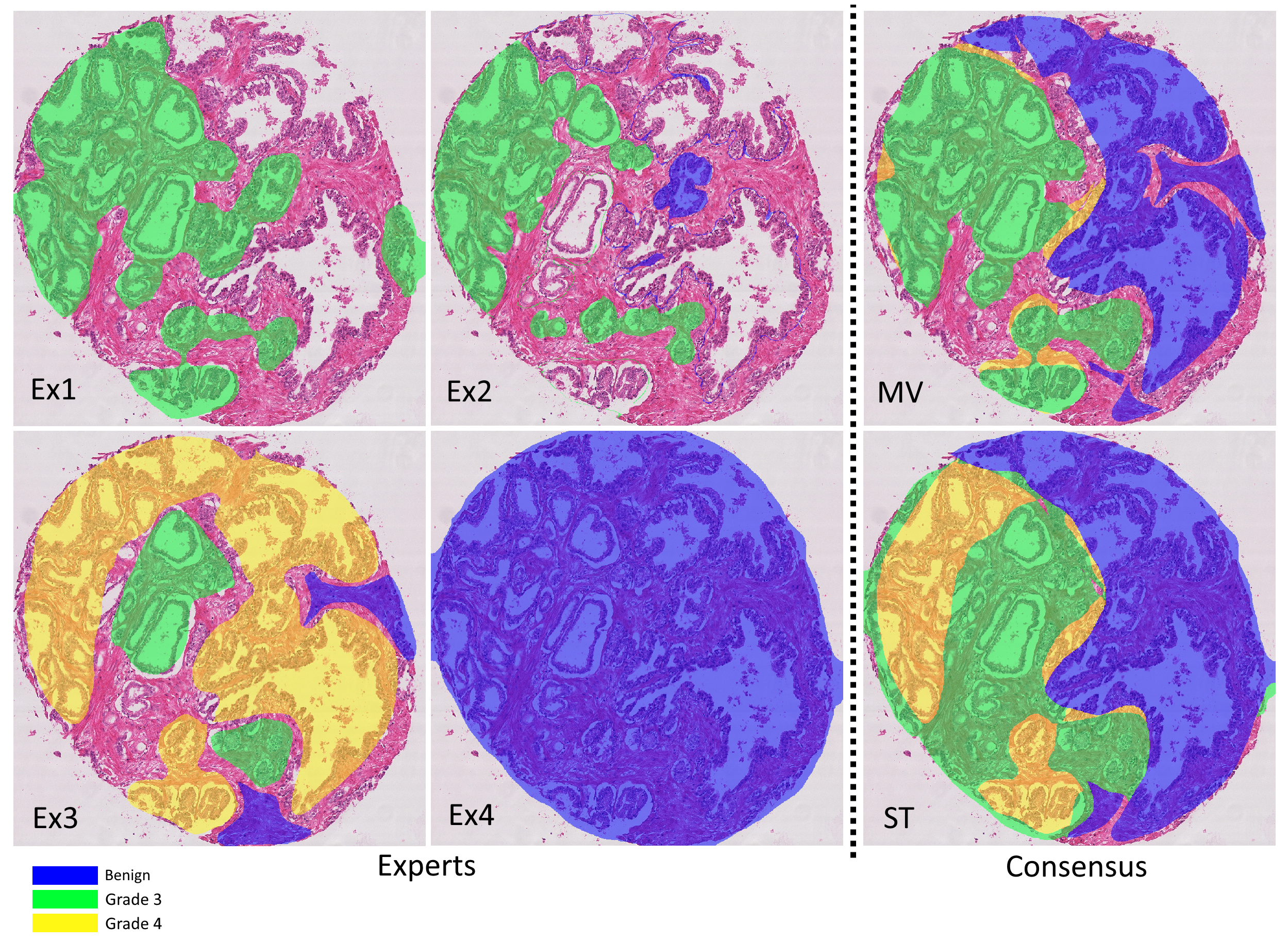
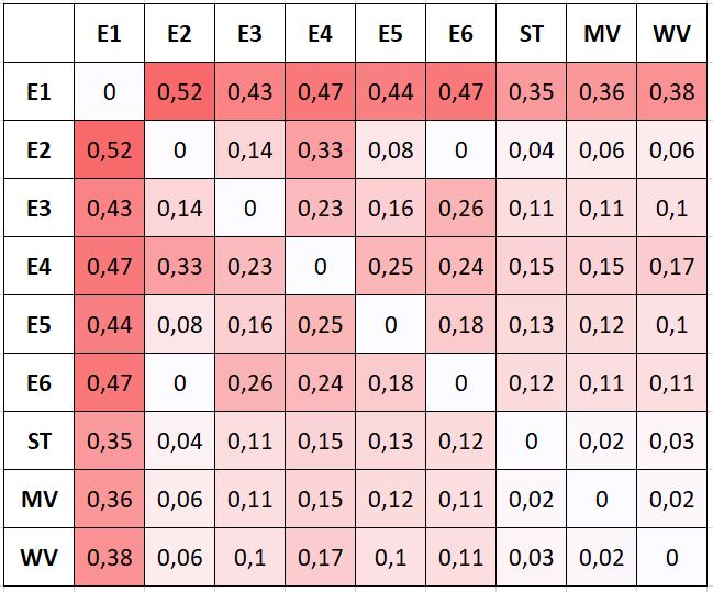
The agreement between the consensus methods (see Table 7.4) is high, although they clearly do not produce identical labels (even at the core level). Once again, the quadratic kappa gives higher values than the unweighted kappa, showing that the disagreements tend to be between adjacent classes. Figure 7.6 illustrates the different annotations provided by the experts, the result of the consensus methods, and the difference that the interobserver variability makes in the computation of the core-level scores depending on the scoring method.
| Consensus | ST | MV | WV |
|---|---|---|---|
| ST | 1. | 0.915 | 0.871 |
| MV | 0.915 | 1. | 0.911 |
| WV | 0.871 | 0.911 | 1. |
|
Consensus |
ST | MV | WV |
| ST | 1. | 0.983 | 0.970 |
| MV | 0.983 | 1. | 0.978 |
| WV | 0.970 | 0.978 | 1. |
These data provide performance ranges to be achieved by the algorithms to produce results equivalent to those of experts. However, the comparison with algorithm performance would not be fair because each expert participated in the consensus. To correct this evaluation and show how that may affect the perception of the results, we compute the agreement levels with a “leave-one-out” strategy consisting in evaluating each expert against the consensus (STAPLE, majority vote and weighted vote) computed on the annotations of all the others.
Our results (Table 7.5) show that all experts, as expected, have a lower agreement with the ground truth when their own annotations are excluded from the consensus. However, not all experts are affected in the same way, and the rankings are not preserved. This shows that the comparisons to a consensus may not reflect the complexity of the relationships between experts.
Expert (N) |
LoO-ST | LoO-MV | LoO-WV |
|---|---|---|---|
| Expert 1 (237) | 0.367 (-0.103) [6] | 0.344 (-0.129) [6] | 0.351 (-0.076) [6] |
| Expert 2 (20) | 0.487 (-0.118) [4] | 0.489 (-0.197) [3] | 0.556 (-0.131) [1] |
| Expert 3 (186) | 0.545 (-0.128) [1] | 0.565 (-0.090) [1] | 0.533 (-0.169) [3] |
| Expert 4 (235) | 0.488 (-0.126) [3] | 0.478 (-0.158) [4] | 0.468 (-0.119) [4] |
| Expert 5 (244) | 0.504 (-0.176) [2] | 0.542 (-0.168) [2] | 0.534 (-0.205) [2] |
| Expert 6 (64) | 0.483 (-0.209) [5] | 0.470 (-0.202) [5] | 0.448 (-0.246) [5] |
Expert (N) |
LoO-ST | LoO-MV | LoO-WV |
| Expert 1 (237) | 0.550 (-0.096) [6] | 0.532 (-0.112) [6] | 0.567 (-0.055) [6] |
| Expert 2 (20) | 0.936 (-0.023) [1] | 0.906 (-0.034) [1] | 0.919 (-0.021) [1] |
| Expert 3 (186) | 0.830 (-0.058) [2] | 0.836 (-0.058) [2] | 0.809 (-0.093) [2] |
| Expert 4 (235) | 0.757 (-0.091) [4] | 0.756 (-0.095) [5] | 0.765 (-0.070) [5] |
| Expert 5 (244) | 0.748 (-0.123) [5] | 0.788 (-0.095) [3] | 0.808 (-0.096) [4] |
| Expert 6 (64) | 0.807 (-0.076) [3] | 0.825 (-0.065) [4] | 0.809 (-0.084) [2] |
7.4.3 Visualizing expert and consensus method agreement
The results shown in the previous tables are averages computed from the head-to-head comparisons between experts, and from comparisons between experts and the consensus “ground truth” obtained with the different scoring methods. MDS allows us to clarify how the experts relate to each other and to the consensus methods, and these latter between them.
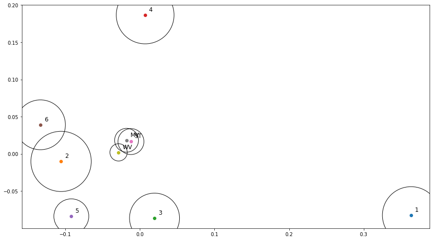
An MDS visualization of the dissimilarity between all experts and consensus methods (of all experts, i.e. not the LoO consensus) is shown in Figure 7.8. The circles are used to represent the average “projection error” of the visualization (i.e. the average difference between the dissimilarity between two measures, reported in Figure 7.7, and the Euclidian distance between the points that represent them). The three consensus methods are very close to each other. Experts 2 and 6 are “identical” in their head-to-head comparison, but their annotations only overlap on a few examples, so their distance to all other points are very different (hence the relatively large circles in the MDS plot). Between the four experts that provided more annotations (1, 3, 4 and 5), Experts 3 and 5 are often in agreement, but Expert 1 clearly appears as an outlier. This latter point is interesting to note because both of the post-challenge publications that used a single expert as their ground truth [6], [42] used Expert 1, indicating that the dataset they used may not be fully representative of a typical pathologist. The lower agreement of Expert 1 with their colleagues was reported in the original publication by Nir et al. [32], but it was computed on “patch-wise grading” (i.e. grading of the pattern present in small patches within each core) instead of the core-level score, leading to a much smaller apparent difference between the experts. As we will more thoroughly explore in Chapter 8, the dataset used in Nir et al. and the subsequent publications by their team are also not exactly the same as the publicly available dataset, making it difficult to compare their results with post-challenge independent publications.
7.5 Discussion
Interobserver variability is an important factor in exploiting digital pathology datasets. When the image analysis task is to reproduce the diagnosis of a human expert, it implies that there is no singular “ground truth” to train machine learning algorithms on, or to evaluate against. This ground truth can be approached through consensus mechanisms, particularly one where pathologists are able to communicate and discuss their difference in opinion. Such a process, however, requires a large amount of time and effort, and therefore makes it very difficult to gather large datasets. Most existing public datasets from digital pathology competitions involve either a single expert, or a small number of experts, leading to a “consensus” that is still likely to contain large uncertainties (as exemplified by the “re-labelling” experiments of, for instance, the AMIDA13 challenge).
Training and evaluating on the consensus annotations may therefore not be the best approach for machine learning, as the information on interobserver variability is thus hidden to the model itself and can only serve as a tool for later discussion. Having access to individual annotation maps brings lots of opportunities for better leveraging this information in the training and in the evaluation process, and to go beyond the “agreement with the consensus” that is typically used as the definitive measure of an algorithm’s performance.
Comparisons between the performance of an algorithm and the performance of “human experts” need to be made carefully. If the comparison is made with a “consensus” annotation, it is necessary to make sure to be fair to both the algorithm and the experts. This can be achieved either through a panel of experts external to the “consensus panel,” used solely for the performance comparison, or through a leave-one-out strategy on the generation of the consensus if an automated method such as STAPLE or majority voting is used.
Our results also show the importance of being extremely precise and detailed when translating rules made for pathologists (such as the ISUP guidelines for prostate cancer grading) into algorithms applicable to machine learning outputs. For the Gleason grading, small differences in the implementation of how to get the Gleason groups from the identified patterns can lead to differences in results. The Gleason 2019 challenge lacks precision in this regard, and this clearly leads to difficulties in interpreting the published results of different researchers, as different assumptions about the data and the task itself are made. This precision is particularly important for competitions, as they typically encourage researchers from outside the specialized field of the task to compete. Gleason 2019 winner Yujin Hu[^52], for instance, states on GitHub[^53] that “I don't quite understand task2, and got it wrong when I participated this challenge,” task2 being the core-level Gleason score prediction task and task1 the per-pixel Gleason pattern semantic segmentation task.
When training on data with interobserver variability, results from Alain Zheng’s master thesis on Gleason grading point to potentially better performances when using individual annotations from all pathologists than when using the consensus only. This, however, required some adequate strategy to focus the final predicted grade on the regions where the per-pixel prediction was more certain.
The evaluation of algorithms based only on agreement to consensus may not give the full picture, particularly if the goal is to compare algorithms with experts. Head-to-head comparisons between experts and algorithms give a more detailed view of the algorithm’s behaviour. This also implies that the results may be more difficult to interpret. The use of adapted visualisation techniques such as MDS can quickly point us towards the potentially interesting insights. This does require some care, however, as there can be large differences between the distances in the MDS visualization and the values in the dissimilarity matrix. It is important to always check the projection error and to always validate any insights with the data in the dissimilarity matrix.
Another clear insight from our studies is that comparing results from post-challenge publications with challenge results is extremely complicated when the test set annotations are not publicly released after the challenge has ended, and when key steps of the evaluation process (such as, for Gleason 2019, the precise method used to compute the core-level scores from the segmented patterns) are not fully described. This encourages researchers to implement their own methods, which will inevitably vary between researchers, leading to performances measured on essentially different datasets. When the challenge has multiple annotations available, the implementation of the consensus mechanism in particular is a really important component to publicly release. Otherwise, it encourages researchers to simplify the problem, leading to the problem in Gleason 2019 of several post-challenge publications choosing to reduce the dataset to the expert most in disagreement with the others only.
Releasing test set annotations and all the code necessary to evaluate results from a set of prediction maps is the only way to remove ambiguities and to ensure that results are reproducible and comparable.
The 3 categories are “,” “,” “” in a 0.196mm² field from the edge of the tumour.↩︎
Corresponding to and .↩︎
The 3 categories are “,” “,” “” in a 0.196mm² field from the edge of the tumour.↩︎
Corresponding to and .↩︎
The authors did not specify which version of the was used.↩︎
https://gleason2019.grand-challenge.org/Home/, June 17th, 2022.↩︎