[Devlog] Getting oriented in anatomical space
Adrien Foucart, PhD in biomedical engineering.
This website is guaranteed 100% human-written, ad-free and tracker-free. Follow updates using the RSS Feed or by following me on Mastodon
Adrien Foucart, PhD in biomedical engineering.
This website is guaranteed 100% human-written, ad-free and tracker-free. Follow updates using the RSS Feed or by following me on Mastodon
During all my PhD, I’ve managed to avoid dealing with the third dimension. I did some work before that on “structure from motion” for detecting trucks from traffic cameras, but that was ten years ago. Now, however, I have to get away from the confort of two-dimensional images, like the digital pathology slides I’m most familiar with, and deal with Computed Tomography, CT in short, images.
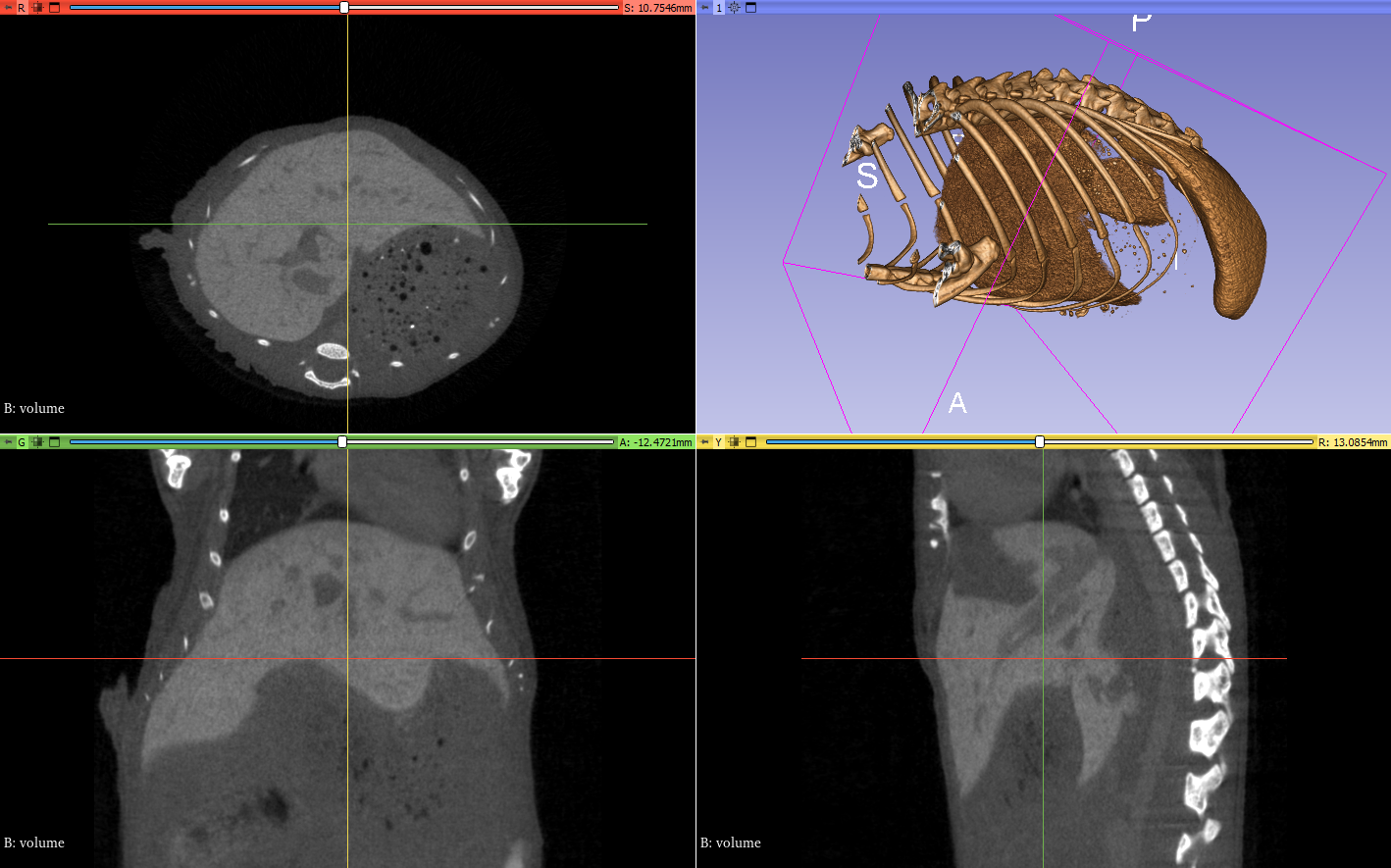
The first question when dealing with CT images is… how to “look” at them? You can use some tricks to get a 3D view of the main elements, but if you want to get the “raw” information, the most common way is to use 2D slices cutting in different directions. I have some CT images of mice, which have been injected with a contrasting agent so that the liver is more visible. Let’s take a quick look using the open source 3D Slicer software:
Since on of the goals of my research is to register ex-vivo histology images to these in-vivo CT, it would be very useful to determine a reliable frame of reference for “anatomical coordinates.” The reason that it’s useful (rather than just looking at voxel coordinates in the volume) is that with CT images, it’s very easy to reorient and/or crop the image in different ways to make it more practical to process in one way or another. A coordinate system that is independent from these transforms is quite useful.
The characteristics that I want for this system are therefore:
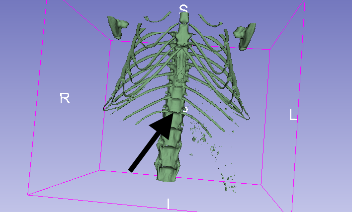
It seems obvious that the reference point, the origin of our coordinates system, will have to be related to the skeleton. The skeleton is very easy to segment, and the position of the different organs relative to the skeleton can be somewhat predictable. As far as my anatomy knowledge goes, also, it should be present and similar in all subjects…
Looking at the images, I think an interesting candidate is the junction between the most posterior ribs and the vertebral column (so the last floating rib from this diagram). In our example image, we can easily find this spot in the 3D view of the skeleton:
So how do we find it automatically?
Let’s start by segmenting the skeleton, using a simple thresholding (it’s fairly easy to find a good threshold automatically in this case, but for simplicity’s sake I’ll hardcode it here). We’ll use SimpleITK to load the volume, but most of the processing will be done with numpy and scikit-image. The useful thing about SimpleITK is that the image object includes information about the “spacing” (the physical size of the voxels).
import SimpleITK as sitk
import numpy as np
%matplotlib inline
from matplotlib import pyplot as plt
path_to_volume = r".\volume.mha"
volume = sitk.ReadImage(path_to_volume)
volume_np = sitk.GetArrayFromImage(volume) # Convert to Numpy array for easier low-level processing
skeleton = volume_np > 100In order to view this skeleton, we can “project” the volume on the three different planes:
plt.figure(figsize=(20,7))
plt.subplot(1, 3, 1)
plt.imshow(skeleton.sum(axis=0))
plt.xlabel('Left <-> Right')
plt.ylabel('Dorsal <-> Ventral')
plt.title('Transverse projection')
plt.subplot(1, 3, 2)
plt.imshow(skeleton.sum(axis=1))
plt.xlabel('Left <-> Right')
plt.ylabel('Anterior (head) <-> Posterior (tail)')
plt.title('Coronal projection')
plt.subplot(1, 3, 3)
plt.imshow(skeleton.sum(axis=2))
plt.xlabel('Ventral <-> Dorsal')
plt.ylabel('Anterior (head) <-> Posterior (tail)')
plt.title('Sagittal projection')
plt.show()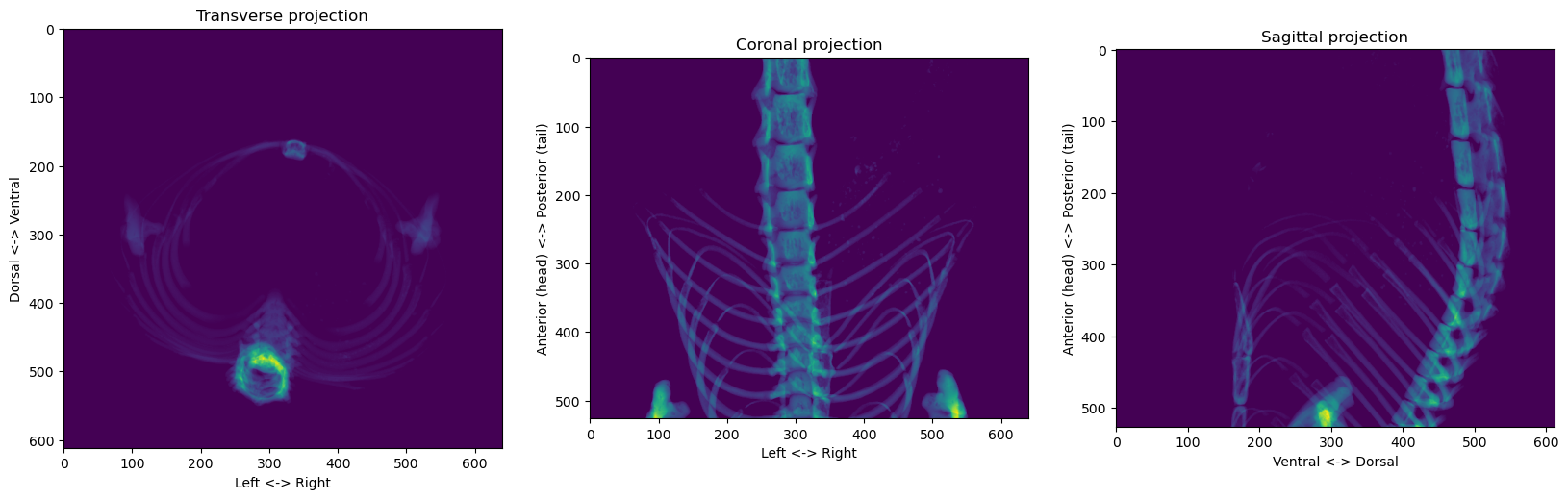
It’s way easier to process 2D images than 3D volumes, so let’s first try to use the coronal projection to find the reference point’s left-right and anterior-posterior coordinates, and we’ll worry about the dorsal-ventral dimension later.
coronal_proj = skeleton.sum(axis=1)

plt.figure()
plt.imshow(coronal_proj)
plt.xlabel('Left <-> Right')
plt.ylabel('Anterior (head) <-> Posterior (tail)')
plt.title('Coronal projection')
plt.show()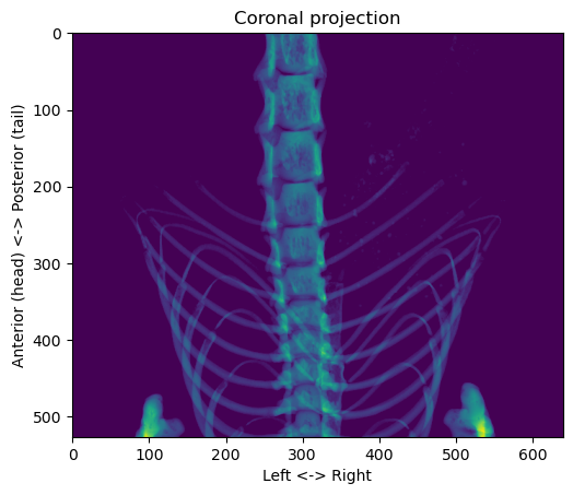
First, we want to find the path of the vertebral column. Since the body is mostly symmetrical in the left-right dimension, we can try to use the centroid of each row to see if it gives us something interesting:
x = np.arange(coronal_proj.shape[1])
centroids = (coronal_proj * x).sum(axis=1) / coronal_proj.sum(axis=1)
plt.figure()
plt.imshow(coronal_proj)
plt.plot(centroids, np.arange(coronal_proj.shape[0]), 'r-')
plt.xlabel('Left <-> Right')
plt.ylabel('Anterior (head) <-> Posterior (tail)')
plt.title('Coronal projection')
plt.show()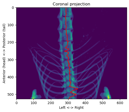
It’s not always well centered because the vertebral column isn’t completely straight, so sometimes just taking the horizontal in this projection is not symmetrical. However, it always remain inside the column, except near the front where the front paws make it more difficult. To adjust for that, we can easily use a “connected components” rule to only keep the largest object in the image:
from skimage.measure import label, regionprops

def select_main_object(binary_array: np.ndarray) -> np.ndarray:
    """Removes any bit that is not connected to the largest object"""
    labels = label(binary_array)
    objs = regionprops(labels)
    max_area, max_area_idx = 0, -1
    for obj in objs:
        if obj.area > max_area:
            max_area = obj.area
            max_area_idx = obj.label
    binary_array[labels != max_area_idx] = 0
    return binary_array

coronal_proj[select_main_object(coronal_proj > 0) == 0] = 0
x = np.arange(coronal_proj.shape[1])
centroids = (coronal_proj * x).sum(axis=1) / coronal_proj.sum(axis=1)

plt.figure()
plt.imshow(coronal_proj)
plt.plot(centroids, np.arange(coronal_proj.shape[0]), 'r-')
plt.xlabel('Left <-> Right')
plt.ylabel('Anterior (head) <-> Posterior (tail)')
plt.title('Coronal projection')
plt.show()
That’s better. Now, we can use a simple heuristic to determine the location on the anterior-posterior axis of the junction that interests us. Looking at the values across the “centroid” line, the local minima correspond to the junctions between the vertebrae. We can then check if there are ribs around that junction, and the first junction with ribs starting from the posterior side corresponds to the target.
from skimage.feature import peak_local_max

centerline_x = np.round(centroids).astype('int')
centerline_value = []
for z, x in enumerate(centerline_x):
    centerline_value.append(coronal_proj[z, x])
centerline_value = np.array(centerline_value)
vertebrae = peak_local_max(centerline_value.max() - centerline_value, min_distance=30)[:, 0]

# To find the first vertebra junction with a rib attached, we look at the variance across the left-right line
# passing through the junction
vertebrae_sorted = np.sort(vertebrae)
xcs = (np.array([np.arange(coronal_proj.shape[1]) for _ in range(len(vertebrae))]).T - centroids[
    vertebrae_sorted]).T
variances = ((xcs ** 2) * coronal_proj[vertebrae_sorted]).sum(axis=1)
z = 0
for idx, variance in enumerate(variances):
    if variance > variances.min()*5:
        z = vertebrae_sorted[idx]
        break

plt.figure()
plt.imshow(coronal_proj)
plt.plot(centroids, np.arange(coronal_proj.shape[0]), 'r-')
plt.plot(centroids[z], z, 'wo')
plt.xlabel('Left <-> Right')
plt.ylabel('Anterior (head) <-> Posterior (tail)')
plt.title('Coronal projection')
plt.show()
For the position in the left-right axis, we want to get in the center of the vertebral column, so we have to adjust the value a little bit:
# adjust x position
maxima = peak_local_max(coronal_proj[z], num_peaks=2, min_distance=50)
x = int(np.round(maxima.mean()))

plt.figure()
plt.imshow(coronal_proj)
plt.plot(centroids, np.arange(coronal_proj.shape[0]), 'r-')
plt.plot(x, z, 'wo')
plt.xlabel('Left <-> Right')
plt.ylabel('Anterior (head) <-> Posterior (tail)')
plt.title('Coronal projection')
plt.show()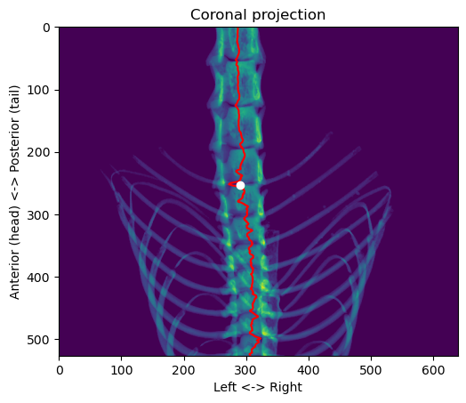
We still have to find the dorsal-ventral coordinates. For that, we can go back to the segmented skeleton volume and take the region in the sagittal projection around the anterior-posterior and left-right coordinates that we found:
region_of_interest = skeleton[z - 15:z + 15, :, x]
y = peak_local_max(region_of_interest.sum(axis=0), num_peaks=1)[0, 0]

plt.figure()
plt.imshow(region_of_interest, cmap=plt.cm.gray)
plt.plot(y, 15, 'bo')
plt.xlabel('Ventral <-> Dorsal')
plt.ylabel('Anterior (head) <-> Posterior (tail)')
plt.title('Sagittal plane')
plt.show()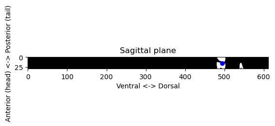
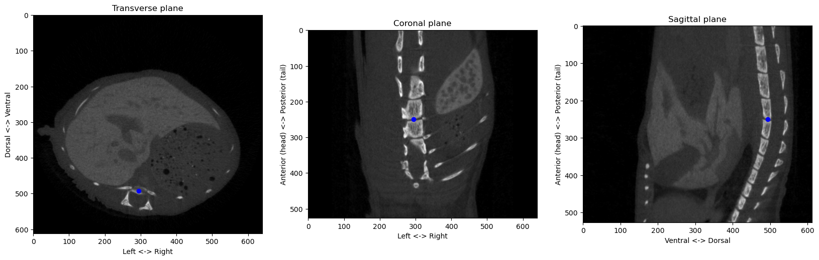
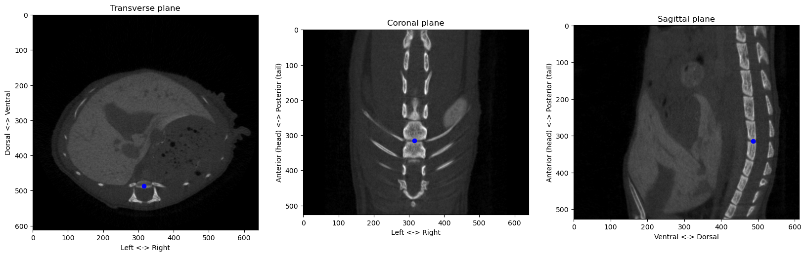
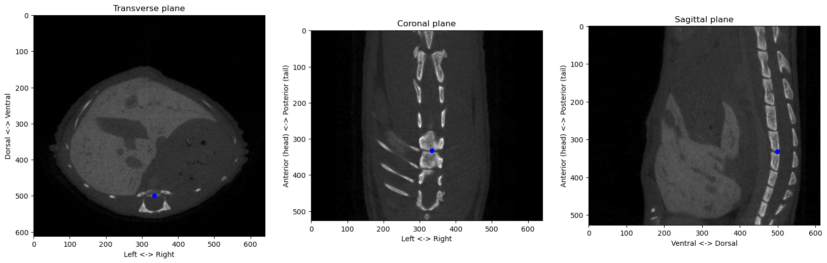
Now we can check where that point is the three planes of our original volumes:
vmin = 0
vmax = 255
plt.figure(figsize=(20, 7))
plt.subplot(1, 3, 1)
plt.imshow(volume_np[z], cmap=plt.cm.gray, vmin=vmin, vmax=vmax)
plt.plot(x, y, 'bo')
plt.xlabel('Left <-> Right')
plt.ylabel('Dorsal <-> Ventral')
plt.title('Transverse plane')
plt.subplot(1, 3, 2)
plt.imshow(volume_np[:, y, :], cmap=plt.cm.gray, vmin=vmin, vmax=vmax)
plt.plot(x, z, 'bo')
plt.xlabel('Left <-> Right')
plt.ylabel('Anterior (head) <-> Posterior (tail)')
plt.title('Coronal plane')
plt.subplot(1, 3, 3)
plt.imshow(volume_np[:, :, x], cmap=plt.cm.gray, vmin=vmin, vmax=vmax)
plt.plot(y, z, 'bo')
plt.xlabel('Dorsal <-> Ventral')
plt.ylabel('Anterior (head) <-> Posterior (tail)')
plt.title('Sagittal plane')
plt.show()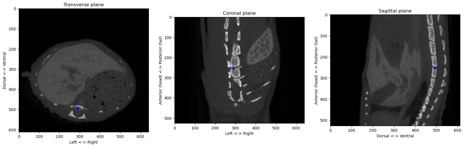
That looks decent enough. With that, we can therefore determine the “origin” point of our system of reference. With the spacing of the volume, we can also compute coordinates in physical spaces along the three anatomical axis:
print(volume.GetSpacing())
spacing = np.array(volume.GetSpacing())
origin = np.array((x, y, z))  # left-right, dorsal-ventral, anterior-posterior
coords_px = np.array((400, 300, 150))
coords_phys = (coords_px-origin)*spacing
print(f"Coordinates {coords_px}px correspond to a point that is \n{coords_phys[0]:.2f}mm right,\n{coords_phys[1]:.2f}mm ventral, and\n{coords_phys[2]:.2f}mm anterior\nfrom the origin at {origin}px, or a distance of {np.sqrt((coords_phys**2).sum()):.2f}mm")
(0.040892000000000005, 0.040892000000000005, 0.040892000000000005)
Coordinates [400 300 150]px correspond to a point that is
4.50mm right,
-7.93mm ventral, and
-4.21mm anterior
from the origin at [290 494 253]px, or a distance of 10.05mmConsolidating all these methods into proper functions and classes, we can check that the algorithms works on different images:
from registration.ct import find_anatomical_reference
from segmentation.ct import skeleton_from_volume
from imagetools.vectors import zyx2vector
from viz.plot import plot_volume_slices
import SimpleITK as sitk

paths = [r"E:\data\PTL\PTL01\Round C1\PTL01_20221220_in vivo\4h\PTL01_20221220_09_1C1G_4H_Rec\volume.mha",
         r"E:\data\PTL\PTL01\Round C1\PTL01_20221220_in vivo\4h\PTL01_20221220_10_1C1D_4H_Rec\volume.mha",
         r"E:\data\PTL\PTL01\Round C1\PTL01_20221220_in vivo\4h\PTL01_20221220_12_1C1G1D_4H_Rec\volume.mha"]

for p in paths:
    volume = sitk.ReadImage(p)
    volume_np = sitk.GetArrayFromImage(volume)
    skeleton = skeleton_from_volume(volume_np, acc_max=1e-5, area_min=1e3)
    origin = find_anatomical_reference(skeleton, zyx2vector(volume.GetSpacing()))
    plot_volume_slices(volume_np, point=origin, figsize=(20,7))