The building blocks of Deep Learning

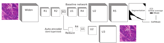
If you read a paper describing a deep learning solution to any sort of problem, you'll probably end up looking at something like this:

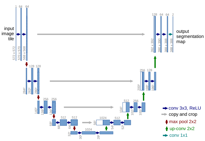
Or this:

Schematic representations of deep neural network allow us to quickly represent very complex structures. The reason we can use those representations and, generally, convey the general idea of what the network does, is that most architectures are made of the same basic building blocks. This allows us to reduce relatively complex operations into a simple "block" or "layer" whose purpose will be well understood by other researchers.

I'll take a look at those blocks in a moment, but first I want to take a magnifying glass into the network to observe the element at the base of all artificial neural networks: the artificial neuron.

The artificial neuron

In 1943, McCulloch and Pitts introduced a mathematical model for the activity of a single neuron [3]. This had a huge influence on the history of artificial intelligence: anything that can be written in a formal mathematical language can be replicated by a computer. If a computer can have individual components behaving like neurons... Why couldn't you have an artificial brain?

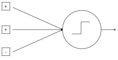
As you can imagine, since it's 2020 and we don't have an artificial brain yet, it turned out to be a bit more complex than that. But the general principle of McCulloch and Pitts' neuron are still valid for modern neural network: input signals (from the "dendrites"), which can have different weights (the "strength" of the connection), positive ("excitatory") or negative ("inhibitory") are summed into a core unit which decides if the signal should be passed on to the output (through the "axon" and into the "synapses").

In an artificial neural network, in general, the structure of the connections (i.e. which neuron is connected to which) is fixed, but the weights of the connections are the parameters that the machine learning algorithm will try to optimize. The structure as well as the activation functions (the function that decides what the output should be based on the aggregated inputs) are hyper-parameters, set by the designer of the solution.

Individual neurons are very limited in what they can do. Connected in large networks, however, they are powerful mathematical tools. Let's start by looking at dense layers.

Dense layers

Dense layers are very easy to explain. All the neurons in the layer are connected to all the outputs from the previous layer, as illustrated below.

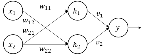
To determine the output of such a network, we can just follow through the connections. If we have two inputs \(x_1\) and \(x_2\), we will have \(h_1 = A_h(w_{11}x_1 + w_{21}x_2)\) as the output of neuron \(h_1\). We can do the same for \(h_2\), then move on to the output: \(y = A_y(v_1 h_1 + v_2 h_2)\). \(A_y\) and \(A_h\) being the activation functions of the different neurons.

One of the key features of neural networks is that the individual operations that are performed in the network are very simple, but we can get very complex outputs (and we can in fact approximate "virtually any function of interest" [4]) by just adding enough neurons to the network.

The problem with dense layers, however, is that the number of parameters grows very rapidly with the number of neurons, and often quickly become impractical. This is particularly true in image analysis. If our input is a 256x256 pixels image, that's already 65.536 input neurons (196.608 if the image is in colours). If we need, for instance, two layers of 1000 neurons each followed by a single output neurons, we will have around 66 million parameters in the model (more than 197 million for colour images). As the general "rule of thumb" in machine learning is that, to train a model, we need "a lot more" annotated examples than we have parameters, this makes things really hard.

Convolutional layers

Convolutional layers are arguably one of the key things that made artificial neural network a practical solution for image analysis rather than a fun curiosity. Convolutional networks first appeared in 1980 with Fukushima's "Neocognitron" [5], but it really became a staple of Deep Learning in 1989 with Yann LeCun's "handwritten digit recognition" solution [6].

The basic concept of convolutional layers is that, instead of connecting every neuron from a layer to every neuron of the next, the connections are limited to a "neighbourhood". If an image passes through a convolutional layer, the output will also be an image, filtered by a "convolutional kernel". The values and size of the kernel will determine the effect of the filter. For instance, in the figure below, we apply a 3x3 kernel designed to get a strong response from horizontal edges.

In a convolutional neural network, each layer will consist in a set of different filters applied to the previous layer.

There are two distinct advantages here, especially for image analysis. The first is that we keep, built into the structure of the network itself, a sense of the spatial organization of the information. With a dense layer, the network has no way of knowing if two pixels are neighbours. Here, the network can extract features starting from neighbouring pixels, and only combining them together at the scale of the image later in the network. The second is that we need less parameters to extract useful information. In a dense network, if we learn a useful local filter at the top-left of the image using 9 connections, we have to use 9 other connections to learn the same filter at the bottom right. In a convolutional network, we learn filters which are applied on the entire image.

For instance, if instead of two dense layers with 1000 neurons, we use two convolutional layers with 64 filters (which will give us about 4 million neurons per layer), we will only need about 40.000 parameters to get what will probably be much more interesting features.

Pooling and upsampling

A downside of convolutional architectures is that neurons lose the overall context of the image, as they can only see a small part of it. It's very difficult to recognize objects, or to perform other high-level computer vision tasks, when every component of the algorithm has a very limited field of view.

Pooling layers are used to downsample an image. This allows the next layer to have a wider field of view, at the cost of a lower resolution. The most common pooling technique is the "max-pooling", which selects the maximum value out of a small neighbourhood and feeds it forward in the network. Pooling effectively summarizes the information contained in a neighbourhood, and makes the network invariant to small translations [7].

Upsampling layers have the opposite effect: they upscale the feature maps, either through a "transposed convolution" operation, or through interpolation. This is typical of segmentation networks, where we need the output to have the same size as the input. Many segmentation network will go through a "downsampling" phase, extracting features with a progressively higher semantic level as the network combines low-level features and puts them into their respective context, followed by an "upsampling" phase, where those features are extrapolated into a "prediction map" giving a class probability for every pixel of the image. This can be seen in both figures 1 and 2 above.

...and all the rest

There are many other types of layers, with more specific purposes. For instance, Dropout units [8] act as a sort of "filter", randomly and temporarily removing neurons of a layer during training. This means that we actually train slightly different, smaller versions of the network in parallel. This has a similar result to training multiple classifiers and averaging their results, which is to make it more likely to generalize well.

Batch normalization is another modifier than we can add to a layer. It standardizes its inputs by estimating their means and variances throughout training. This makes the learning process more stable, and tends to accelerate convergence [9].

Skip-connections are another very common feature of modern deep networks. The idea of a skip-connection is to add shortcuts through the network, where the output from an "earlier" layer is reintroduced later in the network. This can be done over a very short distance, as in residual units [10], which skip a few convolutions, or over large parts of the network as can be found for instance in the U-Net architecture [2].

Conclusion

Network architectures of all sizes and shapes exist, and the state of the art has moved from the relatively short networks of the "early days" of the 00s, with half a dozen layers, to increasingly deep and complex networks with more than a 100 layers in the mid-10s, somewhat moving back to smaller, more efficient architectures in more recent years, as the focus shifted a bit from getting the absolute best performance to getting solutions which can work on regular computers and smartphones for the general public.

There is no doubt that the specific design of the network will influence how well it can model a specific dataset, how well it can perform a specific task, and how efficiently it will be able to learn.

But modern, "general-purpose" networks will work well for a variety of tasks, and more often than not, the most important part of the design process is to think about how to train it. How does a neural network learn? That will be our next topic.

References

1. [↑] Foucart et al., "SNOW: Semi-Supervized, Noisy and/or Weak data for Deep Learning in Digital Pathology", Proc. ISBI 2019. doi:10.1109/ISBI.2019.8759545
2. [↑] Ronneberger et al., "U-Net: Convolutional Networks for Biomedical Image Segmentation", Proc. MICCAI 2015. doi:10.1007/978-3-319-24574-4_28
3. [↑] W. McCulloch and W. Pitts, "A logical calculus of the ideas immanent in nervous activity", Bulletin of Mathematical Biophysics, 1943. doi:10.1007/BF02478259
4. [↑] K. Hornik et al, "Multilayer Feedforward Networks are Universal Approximators", Neural Networks, 1989. doi:10.1016/0893-6080(89)90020-8
5. [↑] K. Fukushima, "Neocognitron: A self-organizing neural network model for a mechanism of pattern recognition unaffected by shift in position", Biological Cybernetics, 1980. doi:10.1007/BF00344251
6. [↑] LeCun et al, " Back-propagation applied to handwritten zip code recognition", Neural Computation, 1989. doi:10.1162/neco.1989.1.4.541
7. [↑] I. Goodfellow, Y. Bengio, A. Courville (2016) "Deep Learning", MIT Press https://www.deeplearningbook.org/
8. [↑] N. Srivastava et al, "Dropout: A Simple Way to Prevent Neural Networks Overfitting", Journal of Machine Learning Research doi:10.5555/2627435.2670313
9. [↑] S. Ioffe and C. Szegedy, "Batch Normalization: Accelerating Deep Network Training by Reducing Internal Covariate Shift", Proc. ICML, 2015. doi:10.5555/3045118.3045167
10. [↑] K. He et al, "Deep Residual Learning for Image Recognition", Proc. CVPR, 2016. doi:10.1109/CVPR.2016.90