How to train your neural network

With all the tools at our disposal now in libraries such as Google's Tensorflow or Facebook's PyTorch, deep neural networks have become increasingly easy to develop, train and use. While this is in general a very good thing, it also makes it very common to treat deep learning algorithms as "black boxes", mysterious beasts which magically transform a "training set" into a trained model with excellent performances on the accompanying "test set". Deep neural networks, however, are only black boxes if we don't open them up and take a peak.

As I've written earlier in the post "Every machine learning algorithm", a "machine learning model" is essentially a function mapping an input (the "data") to an output (the "prediction"). More complex models are characterized by a larger number of parameters in this function. What differentiates a deep neural network from a simple linear model is the much higher complexity of the model which, instead of just being able to find a "straight line" in the space of the input points, is capable of finding essentially any shape. The "shape" in question will be determined by the parameters of the network, which as we've seen in the "building blocks of Deep Learning" are the weights of the connections between the "neurons".

The big question is, of course: how do we find the value of those parameters?

The cost of an error

The first thing that we need to build a training method is a way to determine if an output is correct or not.

Let's go back to our "face detection" problem. The input of our model are the pixel values of a small image patch. The output value is a number representing the probability of the image containing a face.

The "correct output" for the image patches show in Fig. 1 would be: [1, 1, 1, 0, 0, 0] (from left to right and top to bottom). Let's imagine that, for a given set of parameters, our model outputs the values: [0.71, 0.23, 0.55, 0.12, 0.44, 0.05]. What is the "error" made by the model? One thing we could do is just look at the difference between each pair of "expected/predicted" values: 1-0.71, 1-0.23, etc... So, we would get:

Correct output	1	1	1	0	0	0
Model prediction	.71	.23	.55	.12	.44	.05
Error	.29	.77	.45	-.12	-.44	-.05

The mean error would be the average value of this vector (here: 0.15), but it's not a very useful measure. Imagine for instance that we had a completely wrong prediction vector: [0, 0, 0, 1, 1, 1]. The error vector would be [1, 1, 1, -1, -1, -1], for an average of 0. "Positive" errors and "negative" errors are balancing each other, which is not exactly what we are looking for.

The mean absolute error would remove that problem by first taking the absolute value of the error. In our first error vector, this would lead to a cost of 0.35, and in our "completely wrong" example to a cost of 1, which seems a lot more reasonable.

The more commonly used cost functions in machine learning are the mean squared error (for regression problems), and the cross-entropy (for classification problems). Both have the particularity of giving a much higher cost for larger errors (in other words: they consider it's better to be a little wrong most of the time than to be very wrong on rare occasions).

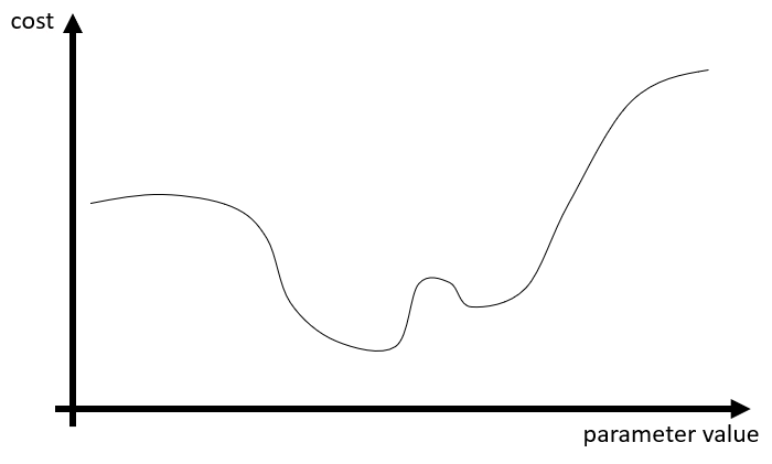
Let's now imagine that we have all the time and computer power we want. We could take every single combination of parameters in our model, and for each of those compute this cost on our training dataset. Whichever combination gives us the lowest "cost" should be the best. If we had only one parameter in our model, we could make a plot showing the cost for every value of the parameter. This would typically look something like this:

Great. But as we don't have all the time and computer power we want, what do we do?

Going downhill

The idea for solving this kind of problem (finding the minimum of a very complex function) comes from all the way to 1847, and a communication to the French Academy of Sciences by Augustin Cauchy [1].

Cauchy's idea is very simple. We start from an arbitrary "position" in this function (meaning in our cases: arbitrary values for all parameters of the model). We can look at the gradient of the function relative to those parameters. In other words: we find the "direction" where moving the parameters makes the function go down.

Now that we have a direction, we move the parameters by a small step, and we start again. Step by step, we go down the cost function, until we hit a point where there is nowhere to go except back up. Then, we know that we've hit a minimum, as illustrated below.

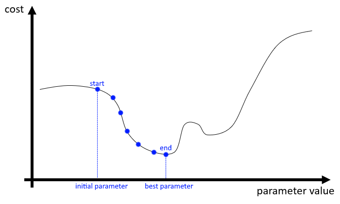
This is the basic process of Gradient Descent. As all parts of a machine learning pipeline, it involves several choices, which will be part of the hyper-parameters. The main choices here are:

• How do we choose the "initial parameters"?
• By how much do we "move" at each step?
• How do we know that we are at the global, not a local, minimum?

The answer to those will depend on the model and the dataset, but in general the initialization will be coming from some form of random generator, the movement will be determined by a learning rate which may vary as the learning progresses, and for the third question, we don't.

How far is too far?

I wrote above that we could in theory find the "best parameters" by computing the cost for every possible value they can take on our training dataset. That was not totally correct. At the very least, it depends on what we define as "best". The minimum of the cost function computed on the training dataset that will give us a prediction as close as possible to the "target" that we gave to the model... But as we've seen in "Every machine learning algorithm", that's not always a good thing.

If our model is complex enough, we can end up basically storing the entire training dataset in its parameters. This leads to a situation where it is perfect at predicting the output for things that is has already seen but has a completely unpredictable behaviour everywhere else. That's overfitting, and as Deep Neural Networks often have millions of parameters, they can easily fall into that trap.

There are things that can be done in the model itself, or in the cost function, to encourage generalization. This is a whole topic by itself which I won't get into: regularization.

But at a most fundamental level, what we really need to do is to evaluate the cost on data that isn't used directly for the gradient descent. When we have a dataset that we want to use for training a machine learning model, we split it in three distinct parts: the training set is used by the model to find the best possible parameters; the validation set is used to evaluate, during the training, how well the model performs on unseen data; and finally the test set is kept aside until the very end, when we have finalized our model, to get a representative measure of how well it actually performs.

Overfitting, within that scheme, is very easy to detect. It happens when the cost keeps getting lower when computed on the training set but starts going up when computed on the validation set. This is a clear sign that we have to stop the training, or risk losing generalization capabilities.

Gradient descent for neural networks

There is one last thing I want to mention before we close this series of articles on the main principles of Deep Learning.

To compute the "gradient" that we mentioned before, we need to be able to formulate the cost function as a function of the parameters of the model, and we need to be able to find its derivative. For a neural network with multiple layers, this is not possible. The relationship between the output and the weights applied in the first layer is far too complex. So what can we do?

In the 1970s and 1980s, the idea of back-propagation for neural networks was developed. Paul Werbos published a version of it in 1982 [2], and the one most commonly cited as popularizing the idea was published in 1986 by David Rumelhard, Geoffrey Hinton and Ronald Williams [3].

A good detailed step-by-step explanation is provided by Michael Nielsen on his website, but the main idea is this:

While it's hard to formulate the gradient with respect to all the weights in the network, it's easy to formulate the gradient with respect to the weights of the last layer. In the back-propagation algorithm, we start by computing those gradients, then we "propagate" the gradients "backward" (hence the title) to the previous layer.

In a sense, it uses the same idea as neural networks in general: instead of solving one very hard problem, we solve millions of comparatively easy problems sequentially, and let the connections between those problems add complexity.

Conclusion

These are the core components of all Deep learning algorithms:

• A robust "pipeline" that transforms the input data into something that the network can handle and interprets its outputs in a way that can be used.
• A network architecture which creates enough complexity, through multiple layers, convolutions, pooling and other operations, to accurately represent the mapping between the input and the output.
• An optimization method, generally based around gradient descent and backpropagation, to set the best weights for the connections in this network.
• A large, good dataset that can provide a reliable source of training, and a good evaluation of the results through the test set.

References

1. [↑] A. Cauchy, "Méthode générale pour la résolution des systèmes d'équations simultanées", in Compte-Rendu des séances de l'académie des sciences, 5 juillet 1847, p536-538 Available online
2. [↑] P. Werbos, "Applications of Advances in Nonlinear Sensitivity Analysis" Available online
3. [↑] D. Rumemhart et al, "Learning representations by back-propagating errors" Available online