Every machine learning algorithm

One of the main things that interested us when our laboratory started working on Deep Learning for digital pathology was to determine which parts of "the deep learning pipeline" actually mattered. Many different Deep Neural Networks have been developed over the years, and in different competitions we often see multiple solutions based on networks which are very similar (or identical) obtaining largely different results [1].

Networks which win high profile challenges are considered state-of-the-art and become wildly used, but it’s not always clear how much of the success (or failure) of a given solution can be attributed to the network itself.

So, before we get into that, let’s take a moment to go through the basics. As we have said before, Deep Learning is a subset of machine learning. Let’s therefore review first what are the main elements of a "Machine Learning" solution, what constitutes the "machine learning pipeline", and what are the building blocks of a Deep Neural Network for image analysis.

Every machine learning problem and algorithm

Any machine learning problem is characterised by a Dataset, a Task, and an Evaluation metric.

The Dataset can take many different forms. It is the "knowledge base" from which we will train our algorithms. In the kind of problems of interest to us here, it will generally be a set of images which may be associated with a set of annotations. The annotations can be very precise (we know what every pixel of the image represent), very imprecise (we know that there is a particular object of interest somewhere in the image), or inexistent. Depending on this level of annotation, we will talk about supervised, weakly supervised, semi supervised or unsupervised datasets, but that’s a topic for later.

The Task is what we want to do with the dataset. Do we want to recognize faces in pictures of a crowd? To count the number of nuclei in a microscopy image? To determine the size and position of a tumour in an MRI?

Finally, the Evaluation metric describes how we are going to decide what a "good result" means for solving our tasks. This may be a harder problem than it looks. Let's take as an example a "face detection" task. The task consists in detecting the location of all the faces in a given image. Let's now say that we have three competing algorithms which obtain the results shown below. Which one is the best?

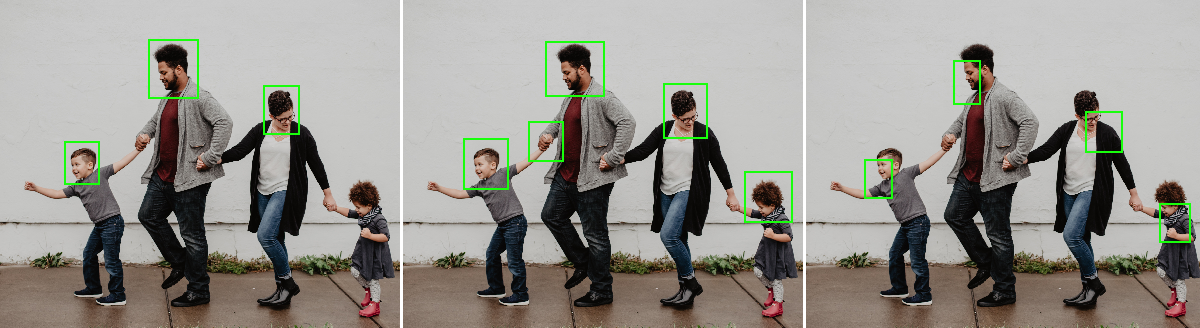
The first one only detected 75% of the faces, but each predicted face is correct. The second detected all faces but added a false prediction. The last one detected all the faces, but the localization is imprecise. The goal of a good evaluation metric is to provide "a quantitative measure of its performance"[2], but different measures will favour different types of performances. If we require a very large overlap between the "true" region of the face and the detected region, the third algorithm will be last, while if we allow approximative localization and simply measure which faces were detected (the sensitivity) and if there were no false detections (the specificity), it may end up being first.

Any machine learning algorithm, conversely, is characterized by a Model with parameters and hyper-parameters, and by an Optimization method.

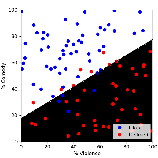
The Model defines the relationship between the input of the algorithm (the data) and its output. Let's go back to our example from our "So... what’s Deep Learning?" post. We were trying to determine if we will like a movie based on the percentage of comedy and the percentage of violence it contains.

One of the most basic models is the linear model. If \(p_c\), \(p_v\) are the percentages of comedy and violence, a linear model would search for a line with the equation \(y = a \times p_c + b \times p_v + c\) that best separates the "movie we like" from the "movie we dislike". \(a\), \(b\) and \(c\) are the parameters of the model. It's what the model will have to learn using the dataset. Running a simple linear classifier such as the Ridge Classifier from the scikit-learn Python library on some fake, generated data would give us something like the figure below.

The hyper-parameters are all the choices that were made while designing the algorithm. A linear model is, for instance, a specific case of a polynomial model, so we could say that the degree of the polynomial model is an hyper-parameter that we have chosen to set at 1.

The Optimization method is the algorithm that we will use to learn the parameters. There are many different ways to go about this, but the main idea is that we will try to adapt the parameters step by step until they are in a position where we can't improve the results anymore. At each step, the algorithm evaluates if each parameter needs to be increased or decreased to get a better result, and by how much, according to the training data. When any change in the parameters seems to give worse results, it stops.

This also requires us to define what "improving" the results mean, which comes back to the question of the evaluation metric. Without going to deep here, it's worth noting that a good evaluation metric for determining if an algorithm is the best at solving a Task isn't necessarily a good metric for optimizing the parameters. As a quick example, any metric that takes a significant amount of time to compute will not be practical for the learning process, as "learning" will generally involve doing millions or billions of such evaluations.

In general, a model with more parameters is said to be more complex. It can potentially solve problems which are more difficult, but at the cost of being harder to train.

To end this chapter, I briefly want to touch on two important notions related to that complexity: underfitting and overfitting. A model is said to be underfitting if it isn't complex enough to accurately represent the data. It is overfitting if it is so complex that it can match the data almost perfectly, which seems like a good thing at first, but is in fact quite problematic. It means that the model has memorized all the examples from the dataset, but isn't capable of generalizing to new examples.

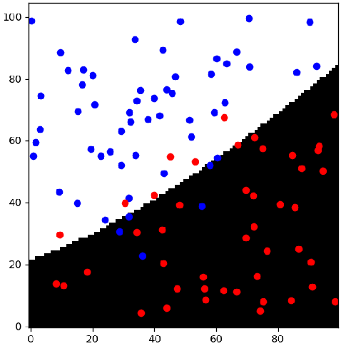
As an illustration, I have trained three different classifiers on the fake "movie" dataset:

• a linear model (trying to fin a straight line that best separates the data), shown in fig. 2 above.
• a third-degree polynomial model (trying to fit a curve of the form \(a \times x^3 + b \times x^2 + c \times x + d\), shown in fig. 3 above.
• a “nearest neighbour” model (attributing the class of the nearest point in the training dataset), shown in fig. 4 below.

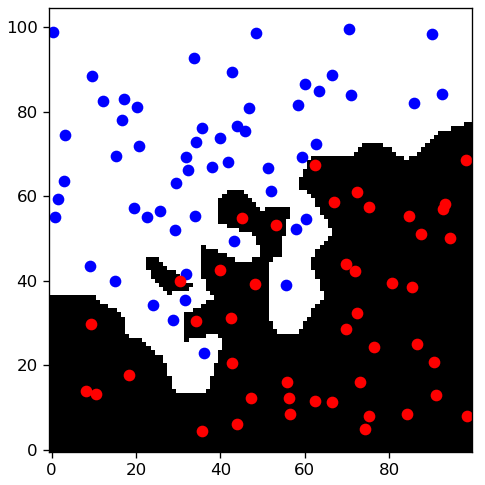
Figures 2-3-4 show the result of the training, with the frontier between the two classes. In the linear and polynomial model, we see that there are points which are on the wrong side of the border. The nearest neighbour, on the other hand, perfectly follows the training set. But is it better?

In the table below, we can see the accuracy (percentage of correct classification) of each model on the training data, as well as on new, previously unseen examples from the same dataset:

Accuracy	Training	Test
Linear	87%	94%
Polynomial	89%	96%
Nearest Neighbour	100%	89%

The nearest neighbour may better represent the training data, but its performance on new examples is the worst of the three. This is a clear sign of overfitting. The difference between the linear and third-degree polynomial is small, but as increasing the complexity improves both the training and the testing accuracy, it's likely that the linear model is underfitting the dataset.

In the next article, we will build on that to look at what constitutes a machine learning pipeline.

References

1. [↑] Aresta et al., "BACH: Grand challenge on breast cancer histology images", Medical Image Analysis 56 (2019). doi:10.1016/j.media.2019.05.010
2. [↑] I. Goodfellow, Y. Bengio, A. Courville (2016) "Deep Learning", MIT Press https://www.deeplearningbook.org/