Cloud'Tech, 2018.
https://doi.org/10.1109/CloudTech.2018.8713350
This is an annotated version of the published manuscript.
Annotations are set as sidenotes, and were not peer reviewed (nor reviewed by all authors) and should not be considered as part of the publication itself. They are merely a way for me to provide some additional context, or mark links to other publications or later results. If you want to cite this article, please refer to the official version linked with the DOI.
Adrien Foucart
Computer-aided diagnosis in digital pathology often relies on the accurate quantification of different indicators using image analysis. However, tissue and slide processing can create various types of image artifacts: blur, tissue-fold, tears, ink stains, etc. On the basis of rough annotations, we develop a deep residual network method for artifact detection and segmentation in H&E and IHC slides, so that they can be removed from further image processing and quantification. Our results show that using detection (tile-based) or segmentation (pixel-based) networks (or a combination of both) can successfully find areas as large as possible of tissue with no artifact for further processing. We analyze how changes in the network architecture and in the data pre-processing influence the learning capability of the network. Networks were trained on the Hydra cluster of the ULB and VUB universities : unfortunately I hadn't taken up the good practice of making code repositories per-publication for easier replicability yet. Some of the code lives on in my deephisto repo, particularly with the ArtefactDataFeed, the ShortRes, the network_train and the artefact utils code. --AF .
Artifacts in histology images are structures which were not naturally present in the tissue but appeared as unwanted byproducts of the tissue processing workflow [1]. In particular, recent developments in multiplex immunohistochemistry (IHC) assays may involve multiple cycles of staining, imaging, chromogen washing and antibody stripping which can strongly and diversely affect the histological slices. However, these multiplex assays enable to better understand and characterize complex pathological processes by shifting from single towards multiple detection of biomarkers on a single tissue slide [2]. Artifacts thus have wildly different causes, morphologies and characteristics, and can be difficult to recognize as such. They can cause potential mistakes in quantitative analyses involving image processing : or, as we've seen in our more recent work, for registration tasks. --AF . Consequently, manual annotations are usually required to identify and to remove the artefactual areas before subsequent analyses. An alternative way can be offered by Deep Learning (DL) methods that are very successful in solving image analysis tasks, including digital pathology ones [3]. In the present study we use rough annotations to train a deep residual network for automatically segmenting artifacts in whole-slide imaging. We propose to work at a relatively low resolution so that the whole slide can be analyzed in minutes, in order to be useful for quality assessment after image acquisition. Our method shows robustness to weak and noisy supervision, which should ease biomedical applications such as in digital pathology. We explore how tweaking the network architecture and the dataset pre-processing affect the results of the algorithm. We compare our solutions with metrics related to the main objective of finding large areas of tissue where we are reasonably certain that there is no artifact : the difficulty of choosing a metric that made sense eventually led us to what became a main topic of my thesis, i.e. the critical analysis of metrics and evaluation methods in digital pathology. --AF .
Proposed artifact detection methods usually focus on one type of defect, such as tissue-folds [4] or blur [5]. These methods use traditional algorithms based on handcrafted features and image statistics. In contrast, DL is a form of representation learning, which includes the feature detection and selection into the learning process. This approach tends to perform particularly well on ill-defined problems, where the objects of interest are difficult to formally describe [6].
DL methods were successfully used in digital pathology for different tasks, such as mitosis localization [7], [8], basal-cell carcinoma detection [9] or breast cancer grading [10]. These methods typically require large supervised datasets. Most of the work in the domain was therefore focused on problems where public datasets with accurate supervision are available, such as the MITOS12, AMIDA13 or MITOS-ATYPIA challenges [8]. These networks typically use a combination of convolutional layers for feature detection, and fully-connected layers for classification. Ciresan et al. use a “cascading” method, with one network to select mitosis candidates (typically, most nuclei), and another more specialized to discriminate between mitotic and non-mitotic nuclei [7].
“Residual units", introduced by He et al [11], allow for faster convergence of large networks, making them particularly useful for training multiple networks in a reasonable time frame without requiring huge GPU clusters. The main concept of residual units is to use an identity mapping to create shortcuts in the network, bypassing the main convolutional layers.
Weak and noisy supervisions have recently become popular research topics. Weak supervision typically refers to supervision that is less precise than the desired output (e.g. image labels to produce pixel segmentation), as in Multiple-Instance Learning [12]. Noisy supervision, on the other hand, refers to cases where the label itself isn’t certain [13].
The datasets consist in tiles from whole-slide images : samples provided by the DIAPath unit of the Center for Microscopy and Molecular Imaging. It was mentioned in the acknowledgements but should really have been put here as well. --AF . Some slides were stained with hematoxylin and eosin (H&E) in a single operation, resulting in few artifacts. Others were manipulated, stained, scanned and washed several times in a multiplex IHC assay to finally produce an hematoxylin and DAB staining image with a large amount of artifacts. Twenty-two slides were included in the training set and three in the validation set. The latter was used for finding the best options in network architecture and dataset processing. Both sets were manually annotated by a non-specialist : specifically, the first author. --AF on the NDP.View2 Hamamatsu software to segment artifacts roughly. One additional slide, showing a different IHC marker evidenced on a different tissue type, was annotated by an histology technologist and kept aside for final testing. Data augmentation is performed with simple axis symmetry, random noise addition on the RGB pixel values and random illumination change.
A whole-slide image can include hundreds of small artifacts and several larger ones (see illustrations in the results). It is therefore very difficult and time-consuming to produce accurate supervision. In such a scenario, we should assume that our supervised dataset is flawed and contains many errors. The annotation errors are of two types: imprecise segmentation (mostly too large regions, with "normal" pixels wrongly annotated as artifacts) and unannotated artifacts : this directly led to the study on imperfect annotation that we started in our ISBI paper. --AF . The first error type is a lesser problem, as removing small tissue areas around the artifacts is better than missing artifacts. The second error, however, may prevent the network from learning what an artifact is : also, the definition of what should "count" as an artifact may vary depending on the application. --AF .
Our dataset is therefore both weak (the supervision isn’t precise) and noisy (the labels aren’t certain). Starting from a standard residual network architecture, we propose different strategies to cope with those issues: using a “fuzzy-target" scheme by applying a Gaussian filter on the target mask so that the supervision includes annotation uncertainty; balancing the dataset to force a certain proportion of the randomly selected tiles to include identified artifacts; comparing the use of detection networks with sliding windows, segmentation networks, and a combination of both.
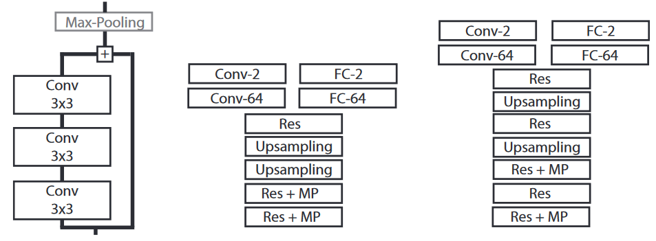
The core network architecture (Fig. 1) is based on “residual” units (with optional downsampling) and upsampling layers to get the last feature maps back to the input image size. We add either two fully-connected layers for artifact detection, or two convolutional layers for artifact segmentation. Every convolutional layer uses a “Leaky ReLU” activation function [14]. A softmax function is applied on the last layer to get the output (either a tile-wise or a pixel-wise prediction). Training is done using the Adam optimizer [15] with the cross-entropy cost function : these choices are somewhat arbitrary and based on "empirical evidence" (fancy for: testing some stuff until it works). Starting from a very simple network, however, did make it easier to test different tweaks more systematically with limited ressources --AF .
The basic architecture is modified in two ways: its size (number of residual units and number of feature maps) and its output (per-tile classification or per-pixel segmentation). Ideally, we want to find the minimal size necessary for the network to get accurate results. As the desired output of the algorithm is a whole-slide segmentation, it makes sense to use a fully convolutional network with a segmentation output. However, given that the annotated segmentation is flawed, it is possible that better results could be achieved with a tile-based classification, which may be less sensitive to the noise : this is justified also by the fact that we typically only "need" to find large areas of tissue without artifact, not to precisely segment the artifacts themselves. --AF .
We test 3 different depths for the “feature learning" part of the network: 3, 5 or 7 residual units (total depth = 13, 19 or 25 layers). These networks are tested each with two different width (64 or 128 feature maps through the entire network), and have either two fully-connected layers added for classification or two convolutional layers added for segmentation.
We want to work at a level of magnification as low as possible, so as to be able to produce the result on a whole slide in minutes at most, while still being able to detect the small artifacts. We try working at 1.25x magnification, 0.625x magnification, or using both in the training set.
We propose to include the uncertainty of the supervision by applying a 2D Gaussian filter on the annotations prior to learning such that the pixels at the annotation borders have “ground truth” values which are not binary. We test the segmentation method with or without this Gaussian filter, and with different standard deviations for the Gaussian kernel (\(\sigma = 2\) or \(\sigma = 6\)).
Artifacts usually constitute a minority class in the images. Moreover, the annotation weaknesses mean that there is a significant amount of unannotated artifacts, especially among the smallest ones. Therefore, if we sample the tiles randomly, we quickly run into a local minimum in our optimization process where every tile or every pixel is classified as “non-artifact.” To avoid that, we balance the training datasets by forcing every batch to contain a certain proportion of tiles with at least some artifact(s) in it. For detection, we test 25%, 50% and 75%. For segmentation (where even tiles with artifacts will have a majority of “non-artifact” pixels), we test 50%, 75% and 100%.
The networks are evaluated at 1.25x magnification. The metrics we measured are: pixel-wise accuracy (Acc), Dice Similarity Coefficient (DSC), True Positive Rate (TPR), True Negative Rate (TNR) and Negative Predictive Value (NPV). Background pixels are excluded from the measures. We add a qualitative measure (Q) which judges whether there is a large enough area of normal tissue left after removing the artifacts (“X” marks a satisfactory qualitative evaluation). As our main objective is to find large areas of artifact-free tissue, we use the TPR and the NPV as main measures of how successful a network is, while removing unsuitable networks according to Q. The DSC was found to be uninformative and is excluded from the result tables for sake of clarity : this qualitative measure was a bit rushed, and clearly lacked a good motivation (and definition). We largely improved on that in a subsequent report. --AF .
The strategy for exploring the impact of the different methodological choices was first to find a “reasonable guess” for a parameter combination that gave decent results. For both detection and segmentation, we started with a Res5 architecture, a tile size of 128x128 pixels, 1.25x magnification, 50% balancing, and sharp targets for the segmentation (networks 4 and 15 in Table 1). We then tweaked each parameter separately to see its effect on the results, keeping the most promising combinations along the way.
The detection networks (D) unsurprisingly tend to wildly overestimate the artefactual regions, resulting in poor accuracies. In contrast, the segmentation networks (S) tend to underestimate artifacts. However, these errors are often due to the rough nature of the annotations: often the prediction of the network more closely match the true shape of the artifact, whereas the supervision includes a lot of normal tissue (Fig. 2). These observations indicate that the segmentation networks generalize well from a weak dataset whereas the evaluation scores do not necessarily reflect this ability because of the poor-quality supervision.
Regarding dataset balancing, higher TPR values are generally obtained when more artifacts are included in the training data for the Res5 detection networks. However, the qualitative evaluation evidences that numerous false positive detections remove too much of the normal tissue when going above 50% balancing. The Res5 segmentation networks do not show such an impact of the balancing strategy, as even networks with 100% balancing see enough examples of non-artifact pixels to properly recognize normal tissue.
Adding lower resolution data (0.625x magnification) tends to produce more false positive detections, as at the lowest resolution most tiles contain some artifacts. For the segmentation networks, this effect is reduced by the fact that most pixels within the tile still are of the non-artifact class. It can actually improve their performance by giving them a slight bias towards artifacts which they tend to underestimate. For the detection networks, however, this means that most of the slide will be classified as an artifact. Using bigger tiles has a negative effect on shallower segmentation networks (Res3), but may have a positive effect on deeper networks (Res5).
The thinner networks (Res3t, Res5t) tend to show slightly lower performances than the others. However, including more layers does not necessarily produce better results. In fact, the performances are almost identical for Res3 and Res5 architectures.
Fuzzy targets (Sf) using a Gaussian filter (\(\sigma = 2\)) produces lower performances for Res3 and Res5 networks, and a slightly better performance for Res7. Using a larger kernel (\(\sigma = 6\)) for Res5 does not decrease the performance as much, without giving better results than the sharp targets (Ss) : this was clearly not a great idea: cross-entropy loss is not well-suited to non-binary labels, as shown eg in this StackOverflow answer. --AF .
We selected two detection and two segmentation networks for the final testing. For detection, after removing the networks with bad Q, the best TPR and NPV are achieved by networks 1 and 4. For segmentation, networks 18 and 21 are kept (see Table 1). We also combined the predictions of the best segmentation and detection networks (4 and 21) by taking the average value of their softmax output. The resulting image is almost as good as the detection networks at finding all artifact pixels, while preserving more of the normal tissue.
| Arch | S/D | Tile | Mag | Bal | Acc | TPR | TNR | Q | NPV | |
|---|---|---|---|---|---|---|---|---|---|---|
| 1 | Res3 | D | 128 | 1.25 | 50 | 81.84% | 88.47% | 81.50% | X | 99.28% |
| 2 | Res5 | D | 128 | 1.25 | 0 | 91.16% | 79.09% | 91.77% | X | 98.85% |
| 3 | Res5 | D | 128 | 1.25 | 25 | 87.56% | 83.53% | 87.77% | X | 99.05% |
| 4 | Res5 | D | 128 | 1.25 | 50 | 79.44% | 90.41% | 78.88% | X | 99.38% |
| 5 | Res5 | D | 128 | 1.25 | 75 | 71.83% | 92.42% | 70.78% | 99.46% | |
| 6 | Res5 | D | 128 | B | 50 | 76.65% | 92.14% | 75.86% | 99.48% | |
| 7 | Res5t | D | 128 | 1.25 | 50 | 80.54% | 85.92% | 80.27% | 99.12% | |
| 8 | Res5t | D | 256 | 1.25 | 50 | 68.03% | 97.56% | 66.44% | 99.80% | |
| 9 | Res7 | D | 128 | 1.25 | 50 | 84.01% | 85.82% | 83.92% | X | 99.15% |
| 10 | Res3 | Ss | 128 | 1.25 | 50 | 95.39% | 47.62% | 97.82% | X | 97.35% |
| 11 | Res3 | Sf2 | 128 | 1.25 | 50 | 96.10% | 36.94% | 99.12% | X | 96.86% |
| 12 | Res3 | Ss | 256 | 1.25 | 50 | 95.73% | 40.02% | 98.74% | X | 96.83% |
| 13 | Res3 | Sf2 | 256 | 1.25 | 50 | 95.80% | 36.60% | 98.99% | X | 96.66% |
| 14 | Res3t | Sf2 | 256 | 1.25 | 50 | 95.94% | 39.46% | 98.98% | X | 96.81% |
| 15 | Res5 | Ss | 128 | 1.25 | 50 | 95.89% | 50.36% | 98.20% | X | 97.49% |
| 16 | Res5 | Sf2 | 128 | 1.25 | 50 | 96.14% | 36.89% | 99.16% | X | 96.86% |
| 17 | Res5 | Sf6 | 128 | 1.25 | 50 | 96.08% | 45.21% | 98.67% | X | 97.25% |
| 18 | Res5 | Ss | 128 | B | 50 | 95.32% | 51.49% | 97.55% | X | 97.53% |
| 19 | Res5 | Ss | 128 | 1.25 | 75 | 95.21% | 46.24% | 97.71% | X | 97.27% |
| 20 | Res5 | Ss | 128 | 1.25 | 100 | 95.49% | 47.26% | 97.94% | X | 97.33% |
| 21 | Res5 | Ss | 128 | B | 100 | 95.19% | 52.44% | 97.37% | X | 97.57% |
| 22 | Res5t | Ss | 128 | 1.25 | 50 | 96.24% | 38.02% | 99.20% | X | 96.92% |
| 23 | Res5t | Ss | 256 | 1.25 | 50 | 95.67% | 45.18% | 98.40% | X | 97.08% |
| 24 | Res7 | Ss | 128 | 1.25 | 50 | 96.21% | 41.57% | 99.00% | X | 97.08% |
| 25 | Res7 | Sf2 | 128 | 1.25 | 50 | 95.86% | 45.44% | 98.42% | X | 97.25% |
| 4 + 21 | 89.77% | 84.45% | 90.04% | X | 99.13% | |||||
The final test is done on a completely different slide annotated by a skilled technician : technologist. Sorry. --AF , and containing a large amount of artifacts with a more precise segmentation than in the training set (see Fig. 2). The results for the selected networks are shown in Table 2. Some details are shown in Fig. 2, and a full-slide view of the results for the combined networks is shown in Fig. 3. As observed for the validation slides, the detection networks tend to overestimate the artifacts. However, both networks preserve enough normal tissue to permit further processing, and many of the “false positives” are due to unannotated artifacts. The segmentation networks do miss some artifacts, but as their segmentation is much more precise they may be better suited if a region of interest for the pathologist is situated near artifacts. The combined solution is, again, a good compromise to keep a bit more tissue than the pure detection network, while identifying almost all artifacts : as we also note in the follow-up paper, this test slide ("Block C" in that description) has a different IHC stain and is from a different tissue type than the training set. --AF .
Processing times for a whole-slide image varied between 1’30” (segmentation only network) and 4’ (combined networks) on an NVIDIA Titan X Pascal GPU.
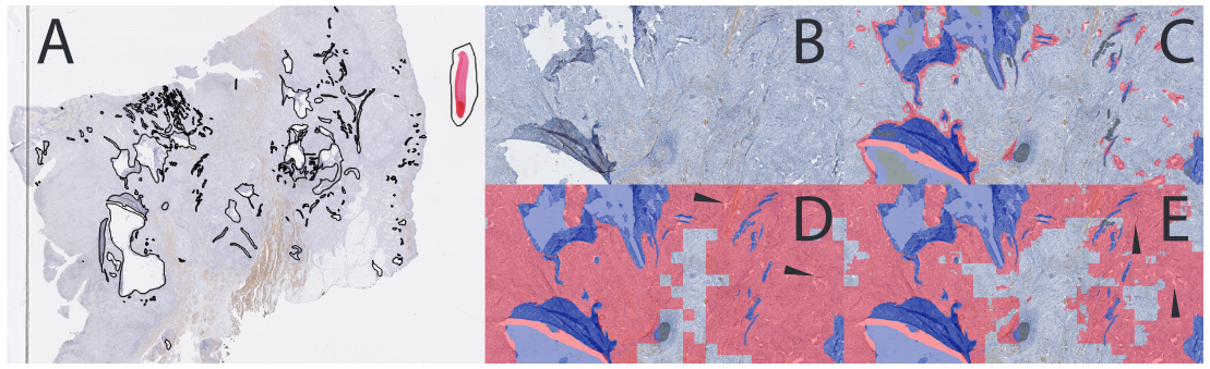
![[full_slide_result] Result on the test whole-slide image for the combined network (4+21).](img/combined-full-slide.png)
| Arch | S/D | Tile | Mag | Bal | Acc | TPR | TNR | Q | NPV | |
|---|---|---|---|---|---|---|---|---|---|---|
| 1 | Res3 | D | 128 | 1.25 | 50 | 84.10% | 87.21% | 83.97% | X | 99.39% |
| 4 | Res5 | D | 128 | 1.25 | 50 | 81.22% | 87.36% | 80.98% | X | 99.38% |
| 18 | Res5 | Ss | 128 | B | 50 | 94.67% | 65.88% | 95.83% | X | 98.59% |
| 21 | Res5 | Ss | 128 | B | 100 | 95.62% | 69.05% | 96.68% | X | 98.73% |
| 4 + 21 | 86.14% | 87.34% | 86.10% | X | 99.41% | |||||
Learning from weak and noisy supervision is a very useful ability for biomedical image processing. In the present study we investigated whether the generalization capabilities of DL methods allow their use when good benchmark datasets are unavailable.
Finding large tissue areas free of artifacts in histological slides is an ill-defined problem where accurate supervision is hard to create. Our DL approach provides good results despite weak supervision. While human annotation tends to miss many small artifacts, our method identifies them even though similar examples are scarce in the dataset. False positives remain common, especially in the “detection” approach, but within acceptable limits for further image processing.
Systematic testing of different choices in the image processing pipeline, in both the DL parameters and the data preprocessing, provides insights into how DNNs can learn from weak supervision. The importance of balancing the training data to ensure proper convergence of the networks is apparent. Combining complementary approaches with opposite biases also helps finding good results: detection networks, which overestimate the objects of interest, combined with segmentation networks, which underestimate them. This combination is advantageous even though the networks are trained separately. Future work should explore the interest of training them together, which may lead to a method closer to the cascading networks proposed in [7].
Our method analyzes a full whole-slide image in a few minutes, possibly serving as both a quality assessment tool and a preprocessing one in the digital pathology workflow : our plans to refine the models and move forward with this tool were set aside as the COVID crisis gave other priorities to our pathologist partners, but it may be revived in the future. --AF .
We gratefully acknowledge the support of NVIDIA Corporation with the donation of the Titan X Pascal GPU used for training the networks used in this study. All the whole slide images were provided by the DIAPath unit of the Center for Microscopy and Molecular Imaging (CMMI), which is supported by the European Regional Development Fund and the Walloon Region [Wallonia-Biomed grant 411132-957270]. C. Decaestecker is a senior research associate with the National (Belgian) Fund for Scientific Research (F.R.S.-FNRS).