December, 2020. Report on Zenodo
: it was initally submitted to Scientific Reports but not accepted, and then I was busy with other papers and ultimately we decided to just let it live as a "report". It did benefit from some peer-review though in the process. --AF
.
https://doi.org/10.5281/zenodo.8354443
This is an annotated version of the manuscript.
Annotations are set as sidenotes, were not reviewed by all authors, and should not be considered as part of the publication itself. They are merely a way for me to provide some additional context, or mark links to other publications or later results. If you want to cite this article, please refer to the official version linked with the DOI.
Adrien Foucart
In digital pathology, image segmentation algorithms are usually ranked on clean, benchmark datasets. However, annotations in digital pathology are hard, time-consuming and by nature imperfect. We expand on the SNOW (Semi-, Noisy and/or Weak) supervision concept introduced in an earlier work to characterize such data supervision imperfections. We analyse the effects of SNOW supervision on typical DCNNs, and explore learning strategies to counteract those effects. We apply those lessons to the real-world task of artefact detection in whole-slide imaging. Our results show that SNOW supervision has an important impact on the performances of DCNNs and that relying on benchmarks and challenge datasets may not always be relevant for assessing algorithm performance. We show that a learning strategy adapted to SNOW supervision, such as “Generative Annotations,” can greatly improve the results of DCNNs on real-world datasets.
In the past decade, Whole-Slide Imaging (WSI) has become an important tool in pathology, for diagnostic, research and education [1]. The rise of digital and computational pathology is closely associated with advances in machine learning, as improvements in data storage capacity and computing power have made both Deep Learning (DL) techniques and WSI processing practicable. DL has become the default solution for solving computer vision challenges, including those in the field of pathology [2].
DL algorithms for image segmentation in digital pathology are generally evaluated through challenges on datasets produced specifically for the competition and often conducted at major biomedical imaging conferences such as MICCAI or ISBI [3]. Those datasets are generally considered “clean,” : even though they often are not, as we discuss in our analysis of digital pathology segmentation challenges --AF using a consensus of annotations provided by multiple experts : which brings its own set of problems, see our SIPAIM21 paper on multi-expert annotations --AF . Producing those datasets, however, is extremely costly and time-consuming, and the datasets available for real-world applications are often not of the same quality [4].
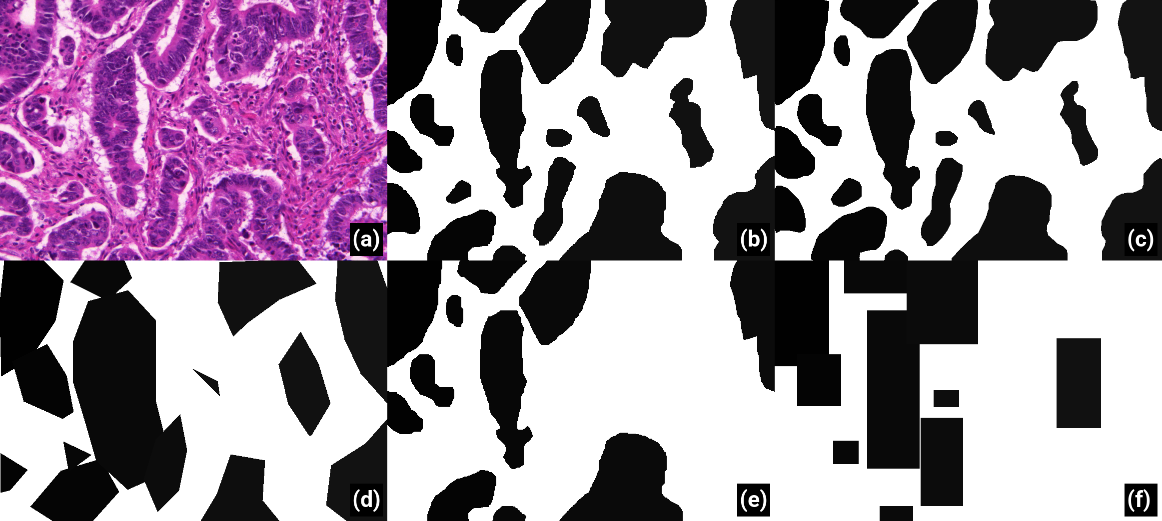
Being able to use imperfect annotations while producing good results is therefore an important challenge for the future of DL in digital pathology. In this work, we focus on annotation problems typically encountered in digital pathology in segmentation tasks that consist in distinguishing a single type of object in a slide image, such as cell nuclei [5], leukocytes [6], glomeruli [7], glands [8] or tumour epithelium [9]. We characterize annotation imperfections using the Semi-Supervised, Noisy and/or Weak (SNOW) concept introduced previously [10] and detailed in the following section. We analyse how these types of imperfection can affect DL algorithms in digital pathology. Then, we explore the capabilities of different learning strategies to mitigate the negative effects of SNOW supervision. For both tasks, we use challenge datasets, considered as perfectly supervised, in which we introduce corruptions of annotations to modulate the quality level of the annotations in a controlled and realistic way, as illustrated in Figure 1. This experimental framework enables us to quantitatively analyse the effects of supervision imperfections and to identify which learning strategy can best counteract them. Our results essentially show that noisy labels due to omitted annotations (Figure 1(c)) have the strongest impact, and that a strategy based on an annotation generator have good potential to provide an effective solution. We then successfuly apply our findings to the real-world task of detecting artefacts in whole-slide images. Finally, we conclude with guidelines to help identify different types of annotation imperfections and appropriate learning strategies to counteract their effects on DL : we should have been a lot clearer here about how this paper differs from the first SNOW publication: it used only one network architecture and one dataset, which didn't make it very robust in terms of the conclusions. Here, we use three different baseline architectures and three datasets with different characteristics. Our analysis of the effects of SNOW is also much more thorough. --AF .
Several datasets are used in this work. First, two clean datasets are used to introduce SNOW supervision and to evaluate their effects in a controlled environment, and then to test different learning strategies to address these effects. A third real-world dataset, targeting artefact detection in whole slides images (WSIs) with supervision imperfections, is then used as a case study and as a test of the most promising strategies. In this section, we present the three datasets and their characteristics. We explain how the annotations are corrupted to simulate the effects of SNOW supervision. We then present the deep convolutional neural networks which are used as baselines. Finally, we describe the learning strategies that are implemented to modify the baseline networks and/or the data pipeline for each of the datasets.
| Data | Tissue | Stain | Training samples | Test samples | Annotations |
|---|---|---|---|---|---|
| GlaS [8] : previously available from Warwick TIA lab, but currently marked as "temporarily not available" on their datasets repository. Copies can be found online, such as on Kaggle, but make sure to cite the original source if you use it... --AF | Colorectal (normal and cancer) | HE | 85 images (around 700x500 pixels) from 16 slides | 80 images (same size) from 16 slides | Gland segmentation |
| Epithelium [11] : tutorial from A. Janowczyk + data available here: http://andrewjanowczyk.com/use-case-2-epithelium-segmentation/ --AF | Breast cancer | HE | 35 images (1000x1000 pixels) | 7 images (same size) | Tumor segmentation |
Table 1 describes the two datasets that are used to introduce annotation imperfections and evaluate their effects in a controlled environment.
It should be noted that the GlaS dataset has a very high density of objects of interest (glands), with 50% of the pixels in the training set being annotated as positive. To be processed by the networks, patches are extracted from the images as detailed in section 2.4.1. Around 95% of extracted patches contain at least some part of a gland (“positive patch”). Comparatively, the Epithelium set has a slightly lower density of positive pixels (33%) with around 87% of positive patches extracted from the images.
Our own artefact segmentation dataset : our dataset is available on Zenodo. Samples provided by the DIAPath unit of the Center for Microscopy and Molecular Imaging --AF is used as a case study of real-world SNOW supervision. It contains 22 WSIs coming from 3 tissue blocks, with H&E or IHC staining, as detailed in Table 2.
| Block | Slide staining | Tissue type |
|---|---|---|
| Block A (20 slides) | 10 H&E + 10 IHC (anti-pan-cytokeratin) | Colorectal cancer |
| Block B (1 slide) | IHC (anti-pan-cytokeratin) | Gastroesophageal junction (dysplasic) lesion |
| Block C (1 slide) | IHC (anti-NR2F2) | Head and neck carcinoma |
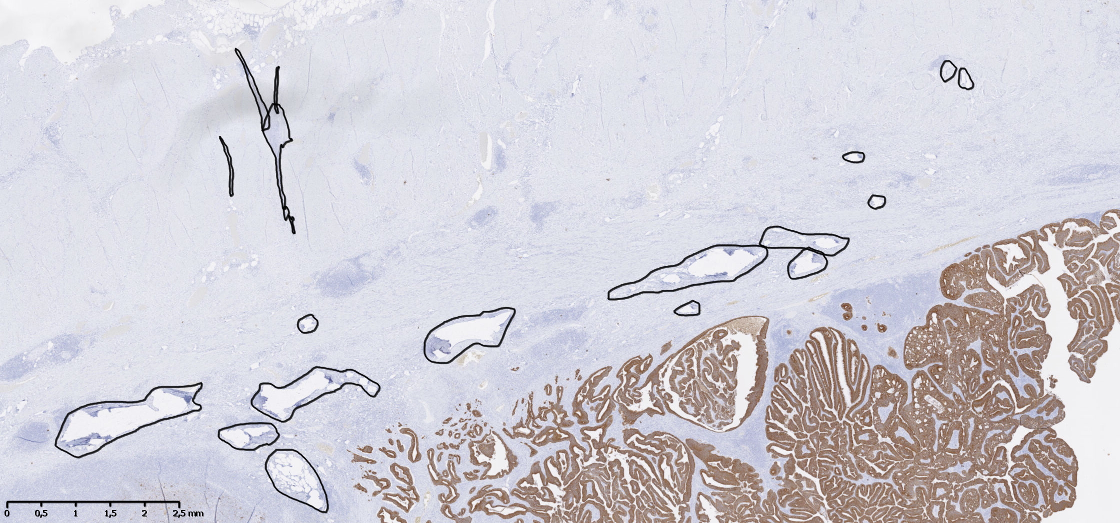
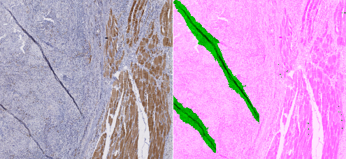
Artefacts in WSIs are very common and heterogeneous in nature. They can be produced at any stage of the digital pathology pipeline, from the extraction of the sample to the acquisition of the image. Some of the most common are tissue folds and tears, ink artefacts, pen markings, blur, etc. [12]. Part of the difficulty of using a machine learning approach is that this heterogeneity makes it hard to annotate the images properly. Our annotations are therefore inevitably imperfect. Objects of interest were annotated quickly with imprecise borders, and many artefacts, especially those of small sizes, were left unannotated (see Figure 2). A total of 918 distinct artefacts are annotated in the training set, with a much lower density of positive pixels (2%) and positive patches (12%) than in the two previous datasets : annotations in the training set were done by me, a non-expert. Block C, however, was annotated more carefully by an experienced technologist, so we could use it in the test set. The dataset splits are described a bit further down. The structure of this paper was reorganized a few times but it's still a bit confusing IMO. --AF .
In addition to our own dataset, we select four slides from The Cancer Genome Atlas (TCGA) dataset [13], which include different types of artefacts [14]. We use these slides to test the generalization capabilities of our best methods.
For each dataset with clean annotations mentioned in Table 1, we introduce random corruptions in the training set annotations mimicking imperfections commonly encountered in real-world datasets (see below). The test set with correct annotations is kept to evaluate the impact of these imperfections on DL performance.
Because creating pixel-perfect annotations is very time-consuming, experts may choose to annotate faster by drawing simplified outlines. They may also have a tendency to follow “inner contours” (underestimating the area of the object) or “outer contours” (overestimating the area). We generate deformed dataset annotations in a two-step process. First, the annotated objects are eroded or dilated by a disk whose radius is randomly drawn from a normal zero-centered distribution, a negative radius being interpreted as erosion and a positive radius as dilation. The standard deviation (
In addition to deformed annotations, we also simulate the case where the expert chooses a faster supervision process using only bounding boxes to identify objects of interest. In this case, we replace each annotation by the smallest bounding box which includes the entire object.
Experts who annotate a large dataset may miss objects of interest. We create what we call in this paper “noisy datasets” by randomly removing the annotations of a certain percentage of objects. A corrupted dataset with “50% of noise” is therefore defined as a dataset where 50% of the objects of interest are relabelled as background (see Figure 1(e)). As there is some variation in the size of the objects, we verified that the percentage of pixels removed from the annotations ranged linearly with the percentage of omitted objects, as detailed in the supplementary materials : available here. --AF .
Different imperfections are also combined: noise with deformations and noise with bounding boxes (see Figure 1(f)), resulting in different “SNOW datasets” which are used in section 4.2 : SNOW generation code can be found on Github, although I don't remember if it's the exact version I used for this paper. I didn't have the good practice of keeping a snapshot of the code per publication when I wrote this one. --AF .
Three different networks are used in this work. First, a short network using residual units similar to those introduced by ResNet [15], labelled ShortRes. As the winner of the 2015 ImageNet challenge, ResNet has become a very popular network for various computer vision, biomedical and other tasks [16]. Residual networks include “short-skip” connections which allow the gradients to flow more directly to the early layers of the network during backpropagation. The second network used is U-Net [17], which is among the most popular architecture in medical image analysis [16]. It includes dropout layers [18] and “long-skip” connections between the downsampling and upsampling layers. The final network, which we call the Perfectly Adequate Network (PAN), combines both short and long skip connections. It is smaller than U-Net, and also combines the outputs from different layers to produce the final segmentation : code for the definitions of the models can be found on Github. --AF .
A schematic representation of the ShortRes and PAN networks is presented in Figure 3. A detailed description of these baseline networks and any variations resulting from the learning strategies detailed in section 2.3.2 is presented in the supplementary materials : available here. --AF . All network implementations are done using the TensorFlow library. The number of parameters for the networks in their baseline version is around 500k (ShortRes), 10M (PAN) and 30M (U-Net). These 3 architectures allow us to study networks with a priori different learning capacities and to measure their respective resistance to different types and/or levels of supervision defects.
![Baseline architectures of the ShortRes (left) and PAN (right) networks. All convolutions and transposed convolutions use a Leaky ReLU [19] activation function. Dimensions along the feature maps are shown for 256x256 pixels input patches and are adapted to other patch sizes.](img/network-architectures.png)
Data Augmentation (always used). In all our experiments, the same basic data augmentation scheme is applied to the training sets that are then used by all networks, left as is (baseline) or combined with one of the learning strategies described below. We modify each mini-batch on-the-fly before presenting it to the network, using the following methods : for an exploration of how much more thorough and realistic data augmentation can help with the GlaS dataset, see our colleague YR Van Eycke's 2018 study in Medical Image Analysis. --AF :
Random horizontal and/or vertical flip.
Random uniform noise on each of the three RGB channels (maximum value is 10% of maximum image intensity).
Random global illumination change on each of the three RGB channels (maximum value of
Only Positive. In this approach, only patches which contain at least part of an object of interest are kept in the training set. Practically, we first compute the bounding boxes of all objects annotated in the training set. During training, we sample patches which have an intersection with these boxes, extended by a margin of 20 pixels on all sides : the (messy) implementation of that is on my Github, eg for the GlaS dataset here. --AF .
Semi-supervised learning. A two-step approach is used for the semi-supervised strategy and is based on the fact that all our networks follow a classic encoder-decoder architecture.
First, an auto-encoder is trained on the entire dataset by replacing the original decoder (with a segmentation output) by a shorter decoder with a reconstruction output, as detailed in the supplementary materials : available here. --AF . The Mean Square Error loss function between the network output and the input image is used to train the auto-encoder, with an L1 regularization loss on the network weights to encourage sparsity.
The second step consists of resetting the weights of the decoder part of the network, and then training the whole network on the supervised dataset. The encoder part of the network is therefore first trained to detect features as an auto-encoder, and then fine-tuned on the segmentation task, while the decoder of the final network is trained only for segmentation. In the experiments on the SNOW datasets reported below, we test two variants of the semi-supervised strategy depending on the supervised data on which the network is fine-tuned: either the full supervised (and corrupted) dataset or only the data used by the “Only Positive” strategy described above.
Generated Annotations. The “Only Positive” strategy may tend to overestimate the likelihood of the objects of interest, especially in cases where they have a fairly low prior (such as in our artefact dataset). We propose a slightly different approach based on a two-step method detailed as follows. First, we train an “Only Positive” network (i.e. using the “Only Positive” strategy) and use it as an annotation generator to reinforce the learning of the final network, which will be trained on the whole dataset in the second step. In this second step, if there are annotations in the image, the final network refers to them as supervision. If there are no annotations, it refers to either this lack of annotation or the output of the annotation generator as supervision. The probability of each possibility should depend on the object prior.
This strategy can be seen as a version of semi-supervised learning because the regions without annotations are sometimes treated as “unsupervised” rather than with a “background” label. But it is also based on label noise estimation. The assumption that positive regions are more likely to have correct annotations results in a highly asymmetric noise matrix, with
Label augmentation. Knowing that labels could be imperfect, especially around the borders, we create slightly modified versions of the supervision via morphological erosion or dilatation (with a 5 pixels radius disk) of the objects of interest that are randomly presented during learning. Following a purpose similar to that of classical data augmentation, this strategy aims at making networks robust to annotation modifications : this is somewhat similar to the "Fuzzy targets" strategy we had tried in our first artifact paper, but trying to avoid the problems of nonbinary labels that we had at that time. --AF .
Patch-level annotation strategies. As mentioned above, typical weak strategies rely on patch-level annotations. However, such strategies are not appropriate for the datasets described in Table 1 because these sets include very few examples of negative patches (5% for GlaS and 13% for Epithelium). This means that with original or noiseless datasets, “weak” networks would see almost only positive examples, whereas with noisy data sets, they would see either correct positive examples or incorrect negative examples. In either case, they will not be able to learn. Therefore, we will not use patch-level strategies in the present work : as we saw with our first artifact paper with the "detection" networks, it does give interesting results for that specific dataset, but since our strategy selection here is based on the results of the Epithelium and GlaS results, it would be weird to include them. --AF .
The networks are trained with patches randomly drawn from the training set images. The patch size is determined for each dataset by preliminary testing on the baseline network, with the goal of finding the smallest possible patch size on which the network can learn. 256x256 pixels patches were selected for the GlaS dataset and 128x128 pixels patches for the Epithelium dataset. To evaluate the results on the test set, images are split in regular overlapping tiles, with 50% overlap between two successive tiles. For each tile, the networks produce a probability map. As most pixels (except those close to the borders) are seen as part of multiple tiles, the maximum probability value for the “positive” class is assigned as the final output. A mask is then produced using a 0.5 threshold applied to this final output. It should be noted that contrary to what is usual in image segmentation, no further post-processing is applied on the results. This aims to avoid contaminating the experiences by external factors but with the consequence of somewhat penalizing our baseline networks compared to what is reported in the literature : validation codes for the different datasets can be found in my PhD dissertation's supplementary Github. Beware, it uses very old TensorFlow code... --AF .
The standard per-pixel F1-score : aka Dice, as it's most often called for segmentation --AF is used as a general purpose metric for both publicly available datasets and their corrupted versions, as the objective of this experiment is not to solve a particular digital pathology task, but to compare the effects of the learning strategies on segmentation accuracy. The per-pixel F1-score is computed for each image of the test set. To determine significant differences between the strategies, in terms of performance achieved with a given training set, the F1-scores obtained on the same test image are compared by means of the Friedman test and the Nemenyi post-hoc test.
On the GlaS dataset, a “statistical score” is also computed to highlight the actual differences in performance between the tested strategies. For each corrupted dataset and for each pairwise comparison, if the difference between the two strategies is judged significant by the post-hoc test (
Eighteen slides (9 H&E, 9 IHC, all from Block A) are used as a training set. The test set is composed of tiles of varying dimensions (between around 400x400 and around 800x800 pixels), extracted from two additional slides from Block A and from the slide from Block B (7 tiles per slide for a total of 21 tiles). Eight of the 21 test tiles have no or very few artefact pixels. The others show examples of tissue tears & folds (6), ink stains (2), blur (2), or other damages.
For each slide and network, we classify the result on each test tile as Good (results are acceptable), False Negative (some artefacts are not detected or the segmented region is too small), False Positive (some tissue region without artefact are segmented), or Bad (completely misses artefacts or detects too much normal tissue as artefacts). Examples of such results are illustrated in Figure 4, where tissue regions considered as correct are shown in pink and those considered as artefactual are shown in green.
To compare the results of the different strategies and networks, we score the predictions on each tile by giving penalties according to the type of error (Good = 0, False Positive = 1, False Negative = 2, Bad = 3). False positives are given a lower penalty than false negative, as it is typically better to overestimate an artefactual region than to misidentify an artefact as normal tissue. We compute the sum of the penalties on all 21 tiles to get a final penalty score, a lower penalty score thus meaning a better strategy : in our first artifact study, we tried using quantitative measures but they were largely uninformative due to the large uncertainty on the labels, so this is actually a much more "objective" measure, even though it starts from a qualitative assessment. --AF .
The last slide from Block C, which is distinguished from the others by the tissue origin and the IHC marker (see Table 2), is used to visually assess the results on a whole slide image in addition to four H&E slides from the TCGA set containing different types of artefact (identified in the “HistoQCRepo” [14]).
For whole-slide prediction, we first perform background detection (i.e. glass side without tissue) by downscaling the image by a factor of 8, converting the image to the HSV color space, and finding background with a low saturation (
In a segmentation problem
: this "Theory" chapter is really badly placed. I don't really remember why we wanted to put it after the materials and methods but rereading it now it doesn't work. --AF
, the instance in a dataset is the pixel. Ideally, perfect annotations for segmentation will provide a correct class for each pixel of each image of the dataset. Let
| Supervision imperfection | Definition and machine learning method | Typical cases in image segmentation |
|---|---|---|
| Incomplete | Label |
Only identified parts of images, or only some of the images in the dataset, are annotated. |
| Imprecise | Label |
The same class is provided for all the pixels of a patch (patch-level annotations). |
| Noisy | Some objects to segment are forgotten. |
The first imperfection type reported in Table 3 occurs when the class information is unknown for a well-identified portion of the dataset. In classical machine learning, semi-supervised methods were developped to process such datasets, mixing labelled and unlabelled data. These methods often use the unlabelled instances to estimate the shape of the distribution, and afterwards the labelled data to separate the distribution into classes [20]. Those methods make the assumptions that samples which are close to each other in the distribution share the same label, and samples which are further away have different labels [21].
The second type occurs when the class information is only provided to groups of instances. In image segmentation, we can have any form of annotation that is less precise than pixel-perfect, such as: patch-level annotations, bounding boxes, polygonal approximations, or points [22][23][24]. Learning methods able to use such imprecise or weak annotations often use the Multiple Instance Learning (MIL) framework [25], in which unlabelled instances are grouped into labelled bags. A typical way of transposing the MIL framework to DL segmentation networks is to use patch-level labels during training with a classification loss, transforming the feature maps of the network into a single class prediction with some form of global pooling [26]. The feature map activation levels are then used to produce a pixel-level segmentation. The feature maps may be combined from different scales and with additional constraints, and these methods have been shown to produce encouraging results in digital pathology [27].
The third and last type of imperfection considered here occurs when all the instances are labelled but with possible class errors. These datasets are described as containing noisy labels. They are typically characterized by a noise matrix (which is usually unknown) giving the probability of two classes being mistaken with each other [28].
As mentioned in the Introduction, we are interested in segmentation tasks usual in digital pathology where only one type of object must be distinguished from the rest. For these tasks it is quite uncommon for an (experienced) annotator to make a “false positive” annotation error, i.e. to label a part of the background as an object of interest. In contrast, “false negative” labels are much more common: some objects of interest may be missed or regions of the image are deliberately not annotated. We can therefore assume that regions around annotated objects of interest are more likely to be correctly supervised than regions far from any annotation. This knowledge can be used in different ways. In [29], the situation of “positive and unlabelled examples” is addressed by first estimating the probability of any unlabelled instance of being positive (in other words, estimating the density of positive examples in the unsupervised part of the dataset). The unlabelled examples are then weighted so that they are treated both as positive and negative examples. Another strategy is to only use the parts of the dataset which are close to positive examples [11]. This means using less training data, but the data used is more likely to be properly supervised.
Real-world datasets in digital pathology show all the types of imperfections described above. Image- or patch-level labels (such as cancer or non-cancer) are relatively quick and easy to get for a large amount of images, whereas pixel-level annotations are difficult and time-consuming [30]. In some digital pathology tasks, the classification of the objects themselves is debatable [31]. More generally in any segmentation problem, the borders of the object may be fuzzy, leading to an uncertainty on the neighbouring pixels. In addition, uncertainty on a label can occur because of a lack of consensus between expert annotators. In fact, the annotation imperfections are intertwined with each other in most real-world digital pathology problems. In a recent study, we brought them together in the concept of Semi-Supervised, Noisy and/or Weak, or SNOW supervision [10]. In that study, we developed an experimental framework to evaluate the impact of SNOW supervision on deep learning algorithms based on convolutional neural networks. We showed that SNOW supervision has adverse effects on Deep Convolutional Neural Networks (DCNNs). However, our results were based on a single network architecture and limited experiments using a single data set, which provided only partial insight into the problem. As detailed below, the same framework is used in the present study for further investigation involving additional datasets, additional (and deeper) networks, as well as additional learning strategies to counteract SNOW effects, in order to draw the most general conclusions possible.
Our experiments with the two “clean” datasets submitted to our annotation corrupting procedure (for the training set only) have several goals. First, they allow us to estimate the extent to which different types of SNOW distorsion make the supervision imperfect. Second, we want to assess the SNOW supervision effects on our baseline Deep Convolutional Neural Networks (DCNNs). Third, we aim to assess how different learning strategies can counterbalance SNOW effects, and finally to infer from the results guidelines for the choice of strategies to be used for different types of annotation imperfection.
We first estimate the extent to which the different types of annotation corruption make the supervision imperfect. For this purpose, we compute the per-pixel F1-Score of different SNOW datasets generated from the GlaS training set with the original set as reference (see Table 4). A low amount of deformation is associated with a 4% loss in the F1-Score. This indicates that when a pixel-perfect segmentation is difficult to define (for instance with objects with fuzzy or debatable boundaries), results based on typical segmentation metrics (F1-Score, Hausdorff distance...) should be interpreted carefully. In such a situation, a difference of a few percent between two algorithms could thus be considered as irrelevant : this is particularly apparent for small objects such as cell nuclei, where a few pixels difference can cause a huge impact on overlap-based metrics such as the IoU or the DSC, as we demonstrate in our 2023 Scientific Reports paper on Panoptic Quality. --AF .
| Dataset | F1 |
|---|---|
| Original (GlaS) | 1.000 |
| 10% Noise | 0.931 |
| 50% Noise | 0.589 |
| Low deformations ( |
0.960 |
| Medium deformations ( |
0.917 |
| High deformations ( |
0.830 |
| Bounding Boxes | 0.836 |
| 50% Noise + HD | 0.455 |
| 50% Noise + BB | 0.557 |
Figure 5 (a) shows the effects of increasing noise levels introduced in the supervision of the GlaS training set on the performance of the 3 baseline DCNNs. Despite their differences in terms of size and architecture, the three networks behave very similarly, with some robustness up to 30% of noisy labels. However, a clear decrease in performance is observed from 40% or 50% of supervision noise.
The effects of annotation erosion or dilatation are much less drastic, as shown in Figure 5 (b), and polygonal approximations seem to have no significant effects (Figure 5 (c)). Bounding boxes can be seen as a such extreme polygonal approximation. Again, the three networks behave in a very similar way with regard to these types of annotation corruption.
![[fig:graph-snow-results] Effects caused by increasing levels of imperfections in the annotations on the F_1-scores for the ShortRes, PAN, and U-Net baseline networks.](img/snow-results-graph.png)
The effects of different types of corruption combined, as mentioned in Table 4, are investigated in the next experiments. We can already conclude that noisy labels have the most negative impact on DCNN performance, in particular from 50% of noise. In view of all these observations, we selected the following corrupted (SNOW) training datasets to test the abilities of different learning strategies to counteract the effects of annotation imperfections:
50% Noise (Noisy)
Bounding boxes (BB)
50% Noise + Bounding Boxes (NoisyBB)
50% Noise + High Deformation (NoisyHD)
Given the very similar behaviours observed above for the three baseline networks with respect to SNOW supervision, only the ShortRes network is used in the first experiments on the GlaS datasets to investigate the effects of different learning strategies. This allows us to draw the first lessons that we then confirm on the Epithelium dataset using the ShortRes and PAN networks, knowing that original versions of both datasets are similar in terms of the quality and nature of the annotations.
As explained in section 2.3.2, we do not include patch-level strategies (considered irrelevant in view of the characteristics of the dataset) in our comparison. The strategies compared to the baseline are therefore:
Only Positive (OnlyP)
Semi-Supervised (with fine-tuning on the full dataset)
Semi-Supervised + Only Positive (with fine-tuning only on the positive data) (SS-OnlyP)
Generated Annotation (GA)
Label Augmentation (LA)
Like the baseline, all of these strategies make use of basic data augmentation. Concerning the Generated Annotation strategy, we had to choose the probabilities of using the annotation generator for the negative patches present in the SNOW datasets. As the original datasets are quite strongly biased towards the presence of objects of interest, we use a probability of either 75% (GA75) or 100% (GA100) of using the annotation generator.
| F1 | Original | Noisy | BB | NoisyBB | NoisyHD | Stat. score |
|---|---|---|---|---|---|---|
| Baseline | 0.841 | 0.231 | 0.724 | 0.511 | 0.212 | -22 |
| OnlyP | 0.836 | 0.768 | 0.730 | 0.697 | 0.660 | 10 |
| Semi-Supervised | 0.831 | 0.467 | 0.756 | 0.522 | 0.207 | -11 |
| SS-OnlyP | 0.819 | 0.729 | 0.740 | 0.730 | 0.428 | 5 |
| GA100 | 0.837 | 0.764 | 0.755 | 0.700 | 0.621 | 12 |
| GA75 | 0.843 | 0.736 | 0.754 | 0.695 | 0.608 | 10 |
| LA | 0.837 | 0.575 | 0.761 | 0.631 | 0.449 | -4 |
Table 5 details the results obtained and Figure 6 illustrates some of them. Surprisingly, these data evidence that the negative effects of the 50% Noisy condition on the baseline network are strongly reduced when using “BB” type annotations. This may be a by-product of the high density of objects in the original datasets. As the bounding boxes cover more tissue area, they may give the networks a bias in favour of the positive pixel class, which helps them get a better score on the uncorrupted test set.
It should be noted that all strategies outperform the baseline, except on the (noise-free) BB dataset for which the differences are not significant. Of the learning strategies tested, three appear to be more effective overall. These are the “Only Positive” and the two “Generated Annotations.” As illustrated in Figure 6, the data in Table 5 should be considered as raw results provided by each learning strategy itself without the beneficial help of post-processing.
To confirm the results reported above, we select the best performing strategies from the GlaS experiment (OnlyP and GA100) to compare with the ShortRes and PAN baseline networks. Regarding the corrupted datasets, we use the 50% noise (Noisy) and the high deformation (HD) sets because there are few differences in the way the different strategies perform against BB deformations. We also include the “Label Augmentation” (LA) strategy to evaluate its effectiveness against high annotation deformations.
The results in Table 6 indicate that regardless of the network, the baseline is only slightly affected by high annotation deformations (combining high levels of both contour simplification and erosion/dilation) and does not benefit from a particular learning strategy in this case. This result confirms that observed for bounding boxes applied to the GlaS data.
| ShortRes | Original | Noisy | HD | PAN | Original | Noisy | HD | |
|---|---|---|---|---|---|---|---|---|
| Baseline | 0.8532 | 0.5447 | 0.8107 | Baseline | 0.8595 | 0.6391 | 0.8283 | |
| OnlyP | 0.8478 | 0.7298 | 0.8078 | OnlyP | 0.8574 | 0.7619 | 0.8263 | |
| GA100 | 0.8480 | 0.6710 | 0.8094 | GA100 | 0.8611 | 0.6806 | 0.8265 | |
| LA | 0.8373 | 0.5768 | 0.8084 | LA | 0.8577 | 0.6480 | 0.8142 |
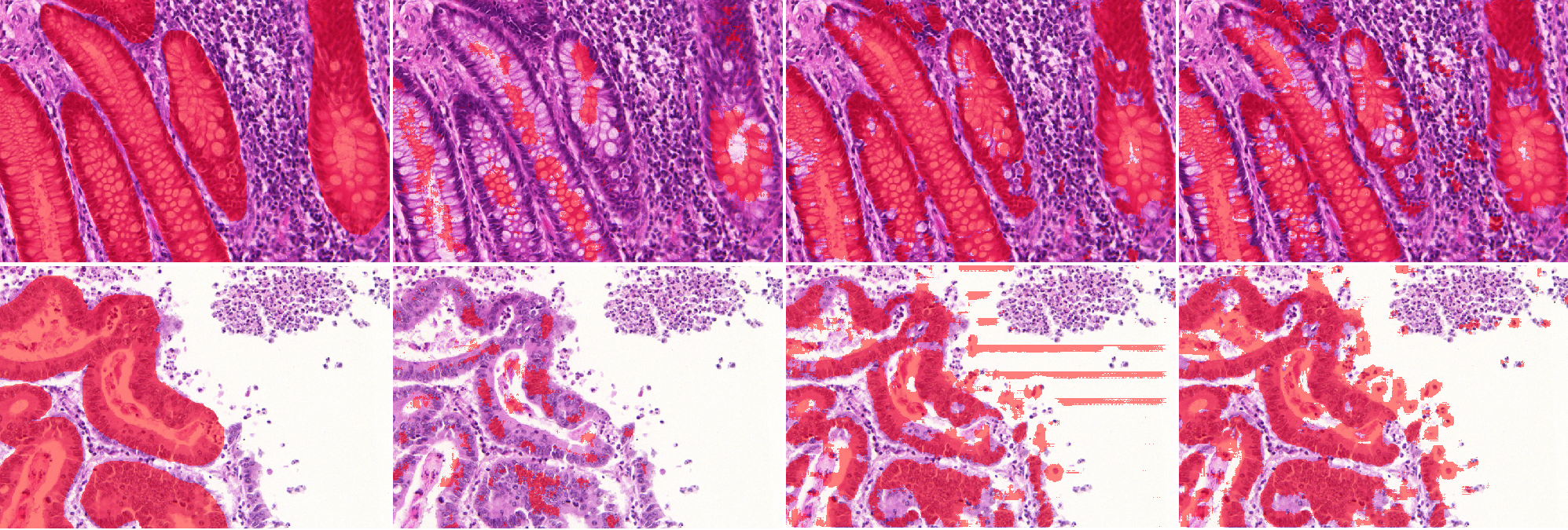
With the original training set and the baseline strategy, ShortRes performs similarly to PAN. With the Noisy training set and the baseline strategy, ShortRes is much worse than PAN but recovers a lot (i.e. 60% of the performance loss) with the OnlyP strategy. With both networks, the OnlyP strategy confirms the good results obtained on the GlaS data and provides the best complexity/accuracy ratio. Using LA does not improve the results, even for the HD training set. Illustrations of these results are provided in Figures 7 and 8. Figure 7 compares the results provided on a test slide by the baseline ShortRes that was trained with either the original, HD or noisy sets. Figure 8 compares the results provided on a test slide by the baseline, OnlyP, GA100 and LA ShortRes networks trained with the noisy set.
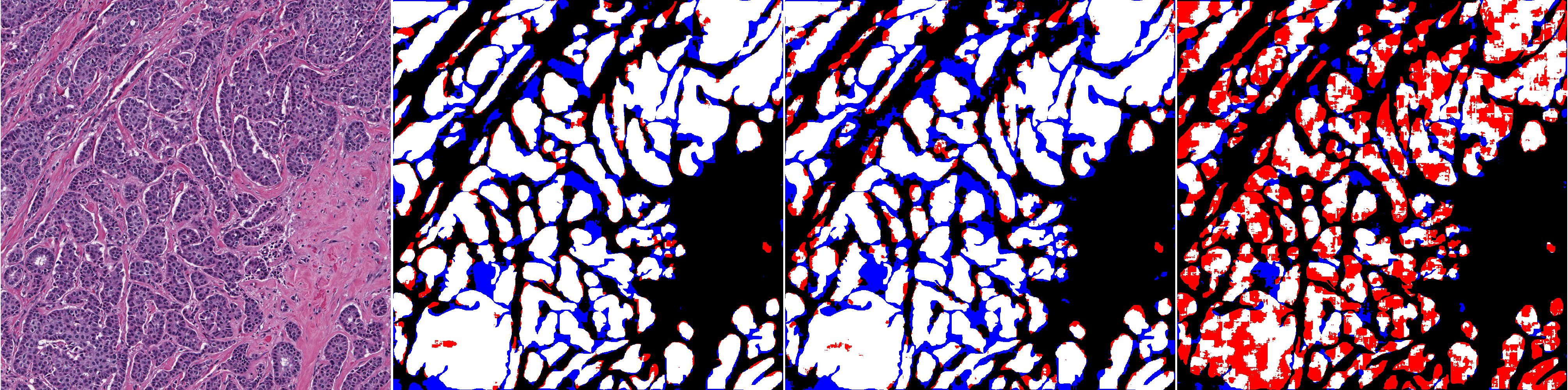
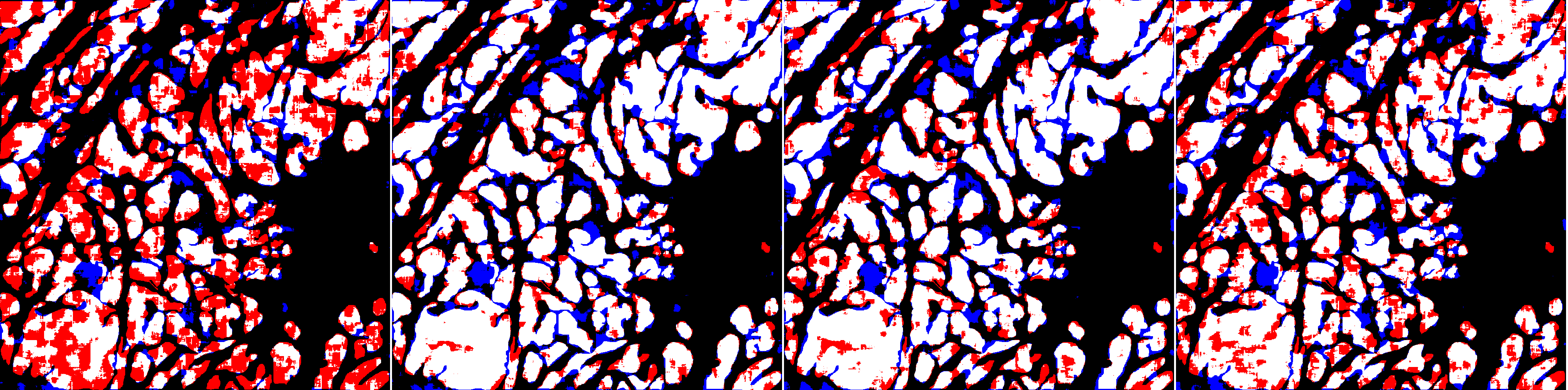
Table 7 shows the results of our qualitative analysis carried out on the test tiles. The GA50 : since the objects of interest are much more sparse here, using GA50 is preferable to GA100. --AF strategy gives the best results with the ShortRes network and confirms its effectiveness with the PAN network. The Only Positive strategy consistently overestimate the artefactual region, with the largest FP number. In this case of low density of objects of interest, the results show that limiting the training only to annotated regions is too restrictive. It should be also noted that for both networks the GA50 strategy is able to retrieve all the “bad” cases from the baseline, which seems less accurate with PAN than with ShortRes.
| ShortRes | Good | FP | FN | Bad | Penalty score |
|---|---|---|---|---|---|
| Baseline | 14 | 0 | 5 | 2 | 16 |
| GA50 | 16 | 1 | 4 | 0 | 9 |
| OnlyP | 13 | 7 | 0 | 1 | 10 |
| PAN | Good | FP | FN | Bad | Penalty score |
| Baseline | 13 | 0 | 5 | 3 | 19 |
| GA50 | 19 | 0 | 2 | 0 | 4 |
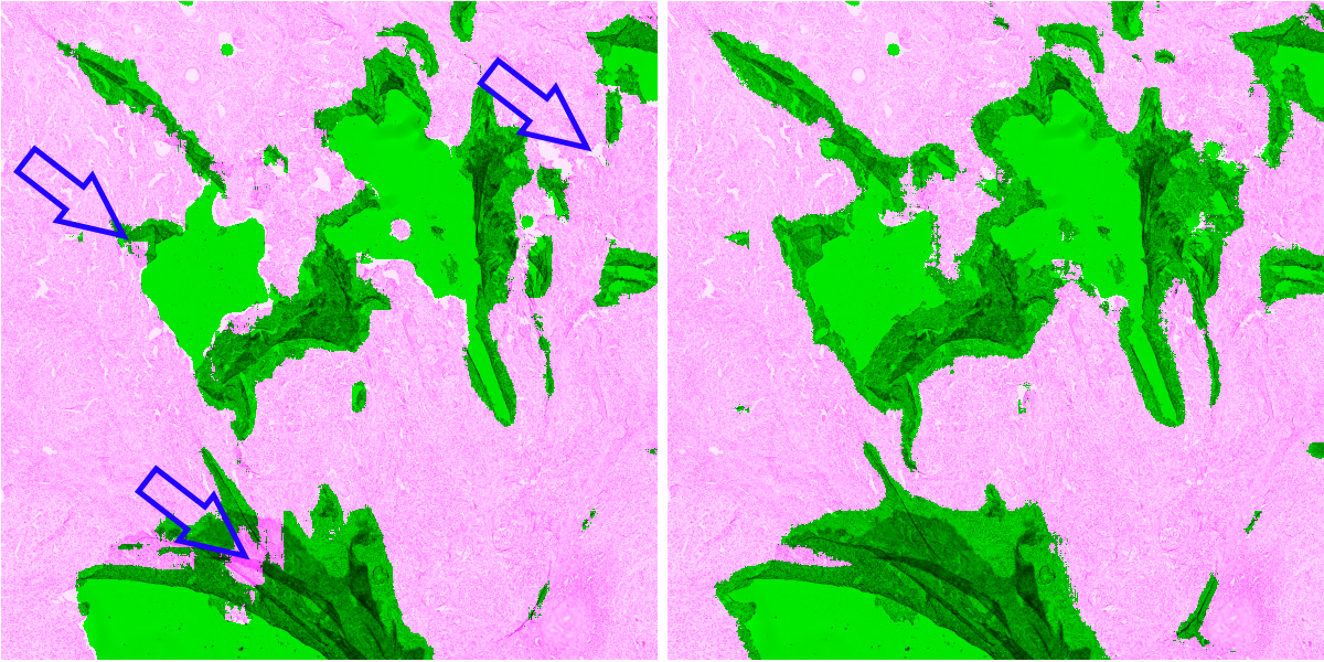
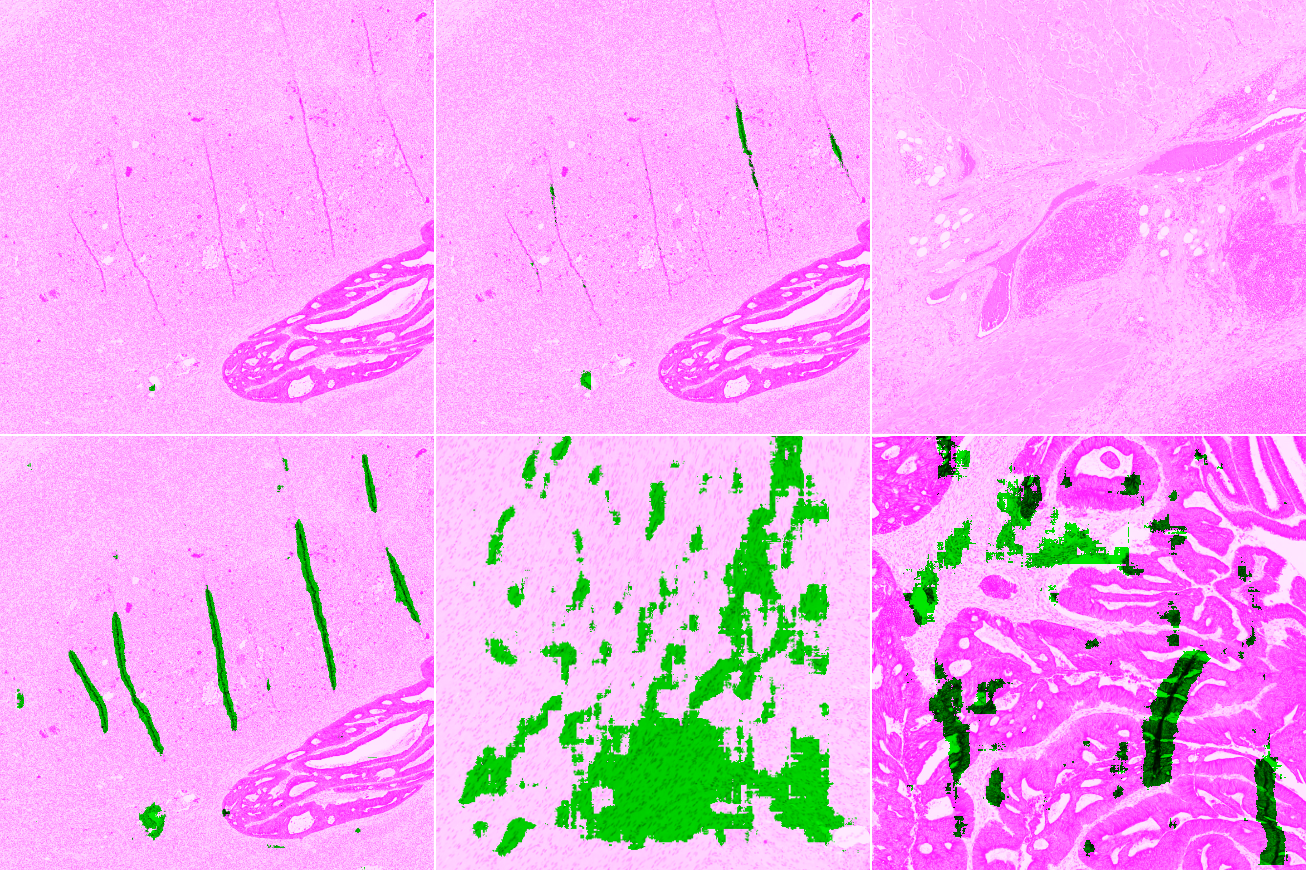
In Table 8, we qualitatively describe the results of the PAN-GA50 network on whole slides. Figure 9 compares the results of the PAN-Baseline and PAN-GA50 networks on part of the Block C slide, with details shown in Figure 10. Other illustrations on the full block C and on TCGA slides are available in the supplementary materials : available here. --AF . It should be noted that the processing time for PAN-GA50 took around 2 minutes 20 seconds for the 4 TCGA slides.
| Slide | (Main) artefacts | PAN-GA50 result |
|---|---|---|
| Block C | Tears and folds | PAN-GA50 misses some small artefacts but its results are generally acceptable. |
| A1-A0SQ | Pen marking | Pen marking is correctly segmented and small artefacts are found. |
| AC-A2FB | Tissue shearing, black dye | The main artefacts are correctly identified. |
| AO-A0JE | Crack in slide, dirt | Some intact fatty tissue is mistakenly labelled, but all artefacts are found and almost all intact tissue is kept. |
| D8-A141 | Folded tissue | The main artefacts are correctly identified. |
In those experiments, we show that SNOW imperfections in the annotations have a significant effect on the results of typical DCNNs. In particular, datasets in which many of the objects of interest are not annotated perform poorly to train networks. In contrast, small to high deformations in the contour of the objects have less impact on the performances of the networks, and no additional strategy make a significant improvement over the baseline. This suggests that, in a real-world setting, it may be better to spend more energy increasing the dataset with quickly annotated contours rather than trying to get pixel-precise annotations. Once the dataset has been done, conversely, it is better to either discard the regions of the images with no annotations, or to include the uncertainty on the labels in the learning process.
The main insights that we draw from the above experiments are as follows: (a) it is important to identify the types of imperfections present in a training dataset in order to use a learning strategy adapted to them; (b) training with a smaller but more accurate dataset performs better than with a larger imperfect dataset; (c) the part of the training dataset with potentially less accurate or missing annotations may be used if we take into account the uncertainty in these annotations and try to address this with an appropriate learning strategy, as we did with the “Generated Annotations” strategies : some extensions of these experiments were also made in Chapter 5 of my PhD dissertation. --AF .
Our results show that a deep learning approach to artefact segmentation can produce interesting results as long as learning strategies adapted to the characteristics of the dataset are used. Artefacts in digital pathology slides are ill-defined objects, which make them particularly challenging to annotate precisely.
Our GA method succeeds in learning from a relatively small set of imprecise annotations, using images from a single tissue type. It generalizes well to new tissue types and previously unseen IHC markers (see Figure 10). This method provides a good compromise between using as much of the available data as possible (as in semi-supervised methods) and giving greater weight to the regions where we are more confident in the quality of the annotations (as in the Only Positive strategy). The baseline method underestimates the artefactual region, as expected from the low density of annotated objects in the dataset. The Only Positive strategy, on the other hand, is too limited in the data that it uses and, therefore, has too few examples of normal tissue to correctly identify the artefacts.
While the PAN network was slightly better than the ShortRes network with the GA50 strategy on the test tiles, it performed worse with the Baseline version. Since ShortRes is significantly simpler (20x less parameters), these observations suggest that for problems such as artefact detection, better learning strategies do not necessarily involve larger or more complex networks.
By using strategies adapted to SNOW annotations, we were able to solve the problem of artefact segmentation with minimal supervision : In Chapter 6 of my PhD dissertation, I amended that to "By using strategies adapted to SNOW annotations, we were able to obtain very good results on artefact segmentation with minimal supervision", as suggested by a member of my jury who rightfully noted that this was a very bold an unjustified claim to make... --AF . Extending the network to new types of artefact should only require the addition of some examples with quick and imprecise annotations for fine-tuning.
In this work, we have shown that the results obtained on clean datasets do not necessarily transfer well to real-world use cases. Challenges typically use complete and pixel-accurate annotations that are often missing in real-world digital pathology problems that must instead rely on annotations with many SNOW imperfections. In addition, challenges typically rank algorithms to identify the best methodology to solve a given type of task. However, it has been shown that these rankings are often not robust to small differences in annotations caused by different annotators [3]. These rankings should be considered even more carefully if the dataset itself may not be representative of the type of annotations that the methodology would encounter in similar real-world applications.
Examining a dataset through the SNOW framework may help reduce guesswork that often accompanies the selection of strategies for solving DL tasks. Our results may also help researchers who need to annotate a dataset to find the most time-efficient method of annotation to achieve adequate results (see flowchart in supplementary materials : available here. --AF ). The first questions to ask when analysing the data are:
What is the density of objects of interest (and of the annotations)? If it is high, is it because the data was cherry-picked and therefore may not be representative of distribution that will be observed in real-world applications? Are all (or most) of the objects well-annotated? In high-density datasets, it may be preferable to limit the training to positive areas only, unless we are certain that the annotations are exhaustive.
How precise are the annotations? Are they pixel-precise? Is “pixel-precise” possible given the nature of the data ? The level of the annotation precision influences both the selection of possible learning strategies and the evaluation. In the case of data with imprecise annotations, evaluations made using quantitative per-pixel measures, such as Dice or Hausdorff, should be interpreted very cautiously. Although our results on datasets with imprecise contours do not show significant benefit for any of the tested strategies, this does not exclude the possibility of processing them more efficiently.
How accurate are the annotations? How much can we trust the class of each pixel? If the annotations are noisy, is it possible to estimate the noise matrix, at least roughly, and integrate this information into the learning process?
Our results have shown that we can improve the performance of DL methods by using a dataset-adapted strategy that takes into account the different aspects of SNOW supervision in annotations, such as the GA50 strategy for the artefact data. The architecture of the network itself, meanwhile, only has a limited effect on the overall results.
Future work should try to incorporate weakly supervised learning strategies using more suitable benchmark datasets into this framework to provide more potential avenues to explore in order to design the best strategy for a given task. While Label Augmentation did not give encouraging results here, the idea of of incorporating contour uncertainty into learning should not be abandoned, and may lead to ways to deal more specifically with the type of imperfection exemplified in our “deformed” datasets. Finally, it would be interesting to study the impact of SNOW annotations in the case of multi-class segmentations [32].