SIPAIM 2021
https://doi.org/10.1117/12.2604307
This is an annotated version of the published manuscript.
Annotations are set as sidenotes, and were not peer reviewed (nor reviewed by all authors) and should not be considered as part of the publication itself. They are merely a way for me to provide some additional context, or mark links to other publications or later results. If you want to cite this article, please refer to the official version linked with the DOI.
Adrien Foucart
Deep learning algorithms rely on large amounts of annotations for learning and testing. In digital pathology, a ground truth is rarely available, and many tasks show large inter-expert disagreement. Using the Gleason2019 dataset, we analyse how the choices we make in getting the ground truth from multiple experts may affect the results and the conclusions we could make from challenges and benchmarks. We show that using undocumented consensus methods, as is often done, reduces our ability to properly analyse challenge results. We also show that taking into account each expert’s annotations enriches discussions on results and is more in line with the clinical reality and complexity of the application : this paper is largely expanded on in Chapter 7 of my PhD dissertation. --AF .
The Gleason2019 challenge [1] is the only digital pathology competition referenced on the grand-challenge.org website which provides detailed annotations from multiple experts in the publicly released training set, as of September, 2021. As such, it offers an interesting opportunity to study how expert disagreement and consensus methods affect our ability to train and evaluate algorithms. In challenges and in comparative studies, algorithms are evaluated against a “ground truth” often provided by experts. Different assessment metrics are often combined to produce a ranking of the algorithms, which has been shown to be highly sensitive to several parameters of the challenge design, including the inter-annotator agreement [2]. In this work we look at how challenges and public datasets aggregate the opinions of multiple experts into a single set of “ground truth” annotations. Using the Gleason2019 challenge as a case study, we analyze how different choices we can make in the way we use and compare multi-expert annotations can lead us to different conclusions. We show that a lot of relevant information about the dataset itself and to evaluate competing algorithms are lost in the aggregation of experts’ annotations into a single ground truth. We further propose guidelines to evaluate digital pathology tasks in a way that is more in line with the clinical reality.
A thorough examination of biomedical imaging challenges has been done in a study by Maier-Hein et al. [2] Analysing 150 challenges organized until 2016, they show that algorithm rankings are greatly impacted by small changes in the evaluation metric, the metrics aggregation method used for ranking, and what is used as a ground truth when multiple expert annotations are available.
A more recent work compiled information on digital pathology challenges [3] and noted that most of them didn’t include adequate information on the methodology used to determine the ground truth of training and/or test images.
The question of how to combine multiple expert annotations into a single ground truth has been studied extensively, comparing simple voting systems, more complex probabilistic models, and end-to-end noisy learning methods [4]–[8]. Practically, however, the available ground truth of digital pathology datasets is often simply produced by a single expert. In the datasets published as part of digital pathology challenges, relatively few described a clear methodology using several experts. The BIOIMAGING2015 challenge [9] discarded the contentious cases, MITOS-ATYPIA-14 [10] aggregated the different experts as an uncertainty on the supervision, and Camelyon disclosed exactly who outlined, inspected, and double-checked the labels [11]. Gleason2019 was the only digital pathology challenge to use the STAPLE consensus [5], and also the only one to fully release the individual expert annotation maps (but only on the training set).
Several experiments have been done on the Gleason2019 dataset to show that training on different consensus methods produced better results than training on a single expert [12]–[14].
In this work, we use this dataset to investigate in greater depth how the exact definitions of consensus and sample scoring methods affect the agreement of experts measured between themselves and with the consensus used as “ground truth.” We show that the relationships between the different experts are more complex than what results from the consensus. However, these relationships are very useful for judging the performance of an algorithm from the perspective of a clinical application.
The Gleason2019 dataset [1] aims at determining Gleason grading based on glandular patterns in Haematoxylin & Eosin (H&E) stained samples. These samples consist of cores in tissue microarray (TMA) slides. Glandular regions are graded from 1 to 5, and a core-level score is computed by summing the two “predominant patterns (by area)” [15]. Throughout this paper, “Gleason grade” refers to the grading of the gland patterns from 1 to 5, and “Gleason score” refers to the core-level aggregated score from 2 to 10. The publicly released training set from the challenge [16] contains 244 H&E stained TMA cores. Six experts annotated some or all of the cores resulting in 3 to 6 annotation maps per core, resulting in 1171 annotation maps. The annotations contain a segmentation of the tumoral glands and their associated Gleason grade. To evaluate the algorithms, the challenge used the STAPLE algorithm [5] as a consensus method to evaluate both the per-pixel grading and the Gleason score computed at the core level. STAPLE uses an expectaction-maximization algorithm which simultaneously evaluate the consensus and the "performance level" of the participants to the consensus. The challenge doesn’t provide a clear heuristic for determining the two predominant patterns and thus the resulting Gleason score, which is usually done visually by the pathologist.
We analysed the training dataset, the only one for which the annotations are publicly available. We compared how both inter-expert agreement and agreement to the consensus are affected by the core-level aggregation method for the Gleason score and by the consensus method. We also looked at different ways of providing a better comparison to algorithm results by a leave-one-out consensus method or by using Multi-Dimensional Scaling (MDS) visualization [17], to gain more insight on the inter-experts and algorithm agreements.
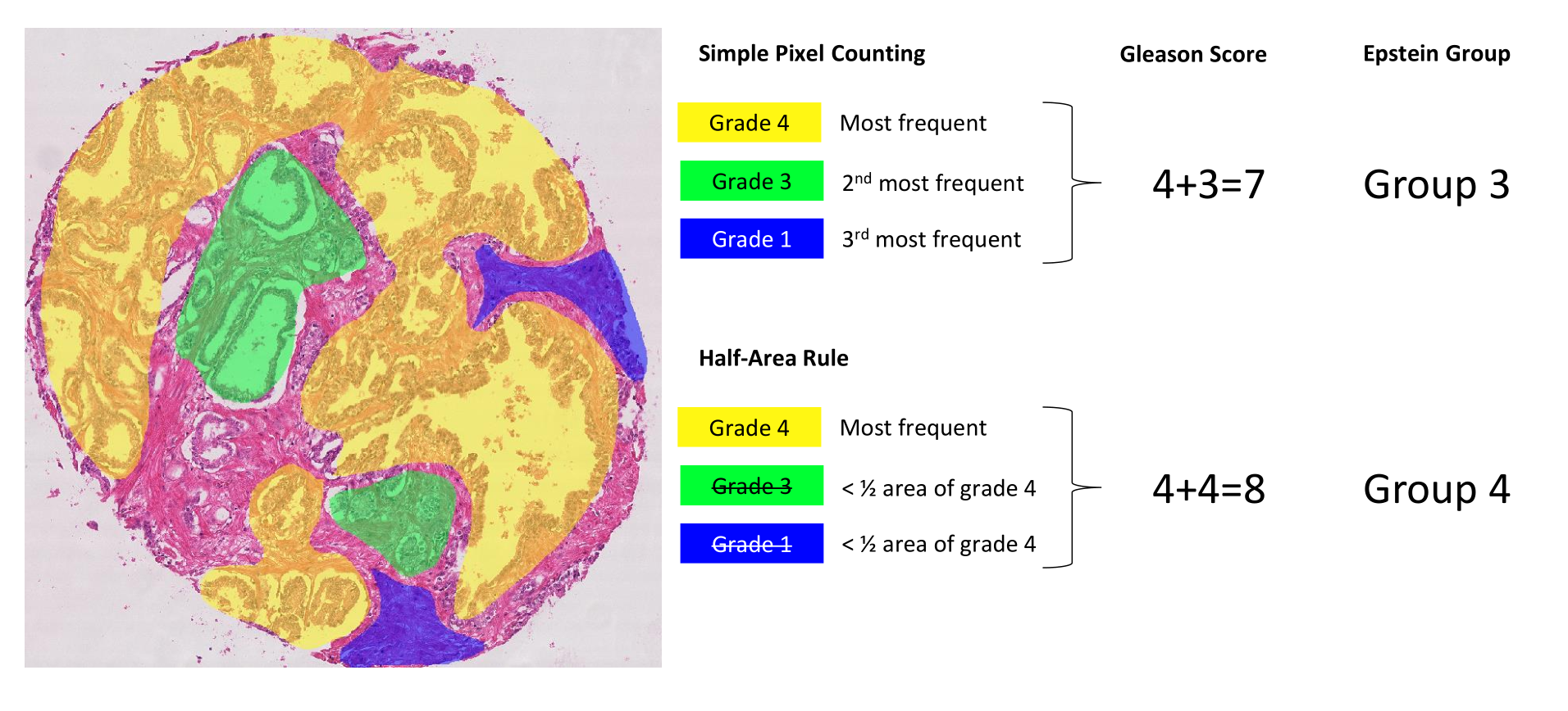
Computing the core-level scores from the annotation maps is not trivial. We propose here two different methods to identify the two predominant patterns. First, a simple pixel counting rule consists in identifying and summing the two most frequent grades in terms of pixels, except if only one grade is present which is then doubled (e.g. a single grade 4 gives a score of 4+4). Second, a “half-area” rule, according to which the second most frequent grade is considered only if the area with this grade is at least half of the area occupied by the first most frequent grade (see Figure 1) : we later realized that this was a little bit too aggressive at removing smaller regions, and replaced it in the PhD dissertation by a heuristic that follows ISUP guidelines more closely, i.e. "consider the secondary pattern either if it has a higher grade than the primary pattern, or if it has a smaller grade and occupies at least 5% of the annotated tumour regions." --AF . This latter rule aims to give more weight to the majority grade and to avoid possible small “contaminations” due to segmentation errors. In addition, we also implement the most recent grouping system used in clinical pathology, i.e. Epstein grouping [18]. This system is also mentioned in the paper describing the challenge dataset and “defines Gleason scores \(\leq 6\) as grade group 1, score 3+4 = 7 as group 2, score 4+3 = 7 as group 3, score 8 as group 4, and scores 9 and 10 as group 5” [1]. Score 3+4 means that there is a majority of grade 3 with some grade 4 present : we also note in the PhD dissertation that we made a mistake here in our handling of "grade 1" annotations, which we correct over there. --AF . The annotation maps containing obvious mistakes (see Section 4) were removed from the dataset so as to not corrupt the results.
The Gleason2019 paper uses the unweighted Cohen’s kappa to measure inter-expert agreement, computed on a patch-wise basis on the Gleason grades. Large studies on inter-expert agreement for Gleason grading by Allsbrook et al. use the unweighted kappa [19] or the weighted quadratic kappa [20], computed on the core-level Gleason scores. As the unweighted and weighted (linear or quadratic) kappa indices all behave differently with regards to the number of categories, this study will focus on the unweighted kappa only. It should however be noted that the agreement metrics is another potential source of bias in the interpretation of published results, particularly if its exact definition is not provided.
The Multi-Dimensional Scaling (MDS) visualisation is produced by computing a dissimilarity measure (here defined as 1-kappa) on all head-to-head comparisons. The dissimilarity is used as a distance metric, and MDS creates a two-dimensional projection where those distances are preserved as much as possible and shown as Euclidean distance on the plane. Each projection is surrounded by a circle whose radius corresponds to the precision of this projection and is computed as the average of the differences between the dissimilarity between a point and each other point and the corresponding projected distance on the plane.
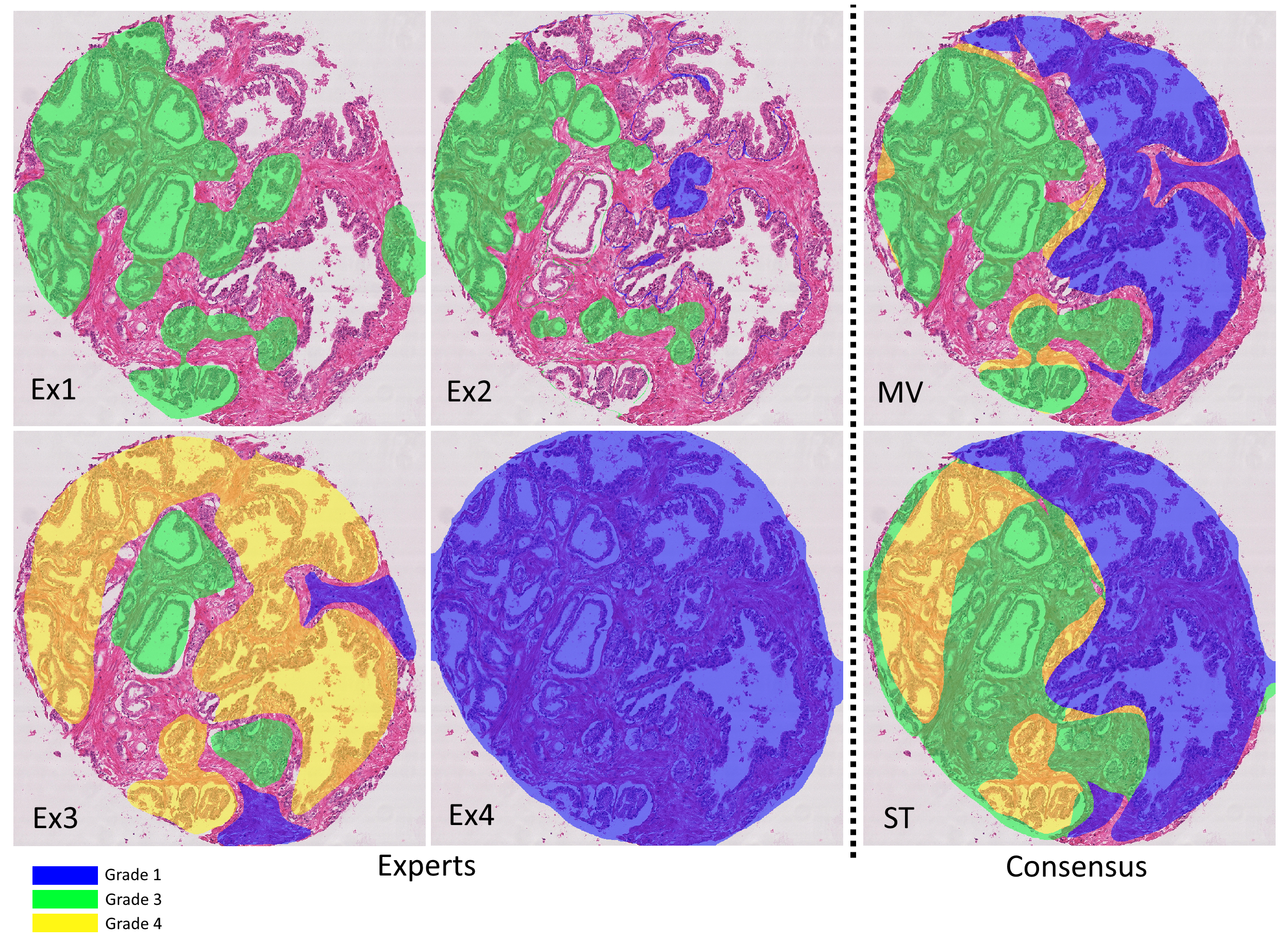
As described above, the Gleason2019 publicly released training dataset contains 244 H&E-stained TMA cores annotated by 3 to 6 expert pathologists. These maps show a large variability between the experts. In addition, many of the provided annotation maps also have clear mistakes. As others noted [21], some of the annotated contours were not closed properly, leading to glands labeled as “background” (corresponding to glass slide and/or stroma), whereas the expert clearly intended to grade them. Figure 2 shows the variability of the annotations for a single core, as well as an example of a clear mistake in one of the maps. From our analysis, about 15% of the annotation maps have this issue (185/1171), most of them coming from the same expert. More disturbing, it is unclear whether this problem also appears in the test set, as these annotations weren’t made public : the results of the challenge as published on their website are also problematic, as I explain in Chapter 8 if my dissertation. The organizers of the challenge have not responded to my requests for clarification, and the results of the challenge were not published (as of today) in a journal. The winners of the challenge have published their results (Qiu et al.), but they are clearly as confused as I am by what the published results actually mean, with the confusion matrix being presented at the same time as related to "core-level predictions" and then as showing percentages of correctly classified pixels. --AF .
While the challenge is partially evaluated on the Gleason score of each core (see Section 3), these core-level scores are not provided with the training set. Similarly, while the participants are evaluated against the STAPLE consensus maps, these latter are not provided along with the individual maps.
These uncertainties have led authors to use different strategies when using the dataset. Khani et al. noted the mistakes in the annotations, corrected them manually and used the STAPLE consensus as a ground truth for training and testing [21]. We did not find any other publication mentioning these mistakes explicitly. The ground truth used by others varied between the STAPLE consensus [22], a simple majority vote [23], using a single expert [24] or merging the different annotations into a “grade probability map” [25].
In the paper introducing the Gleason2019 dataset [1], the authors report the unweighted Cohen’s kappa between experts, computed on a “patch-wise” basis, which is found to range from 0.36 to 0.72 in one-to-one comparisons. These scores are compared to [19], which reports an overall (averaged) kappa of 0.435 between 41 general pathologists and a “consensus” produced by urologic pathologists in [20], which itself reports an overall weighted quadratic kappa (which is systematically higher than the corresponding unweighted kappa) with a range of 0.56-0.70. Allbrooks’ studies, however, computed the agreement based on the core-level Gleason score (as we do below), while the Gleason2019 study reported a patch-level Gleason grade.
We computed the unweighted kappa for all inter-expert agreements using the Gleason scores (ranging between 2-10) and the Epstein groups (ranging from 1-5), using the simple pixel-sum and the half-area rule. Our experiment (see Table 1 : see updated/corrected version of the table (Table 7.2 in my PhD dissertation). Also includes quadratic vs weighted kappa. --AF ) shows to what extent the results vary depending on the scoring method. The average kappa values range here from fair (.2-.4) to moderate (.4-.6) agreement depending on the scoring method. The individual head-to-head comparisons (see ranges) vary from slight (.0-.2) to substantial (.6-.8), with a perfect (1.) agreement between experts 2 and 6 in the case of the Epstein grouping. However, these two experts have very few annotation maps in common and their head-to-head comparison only concerns 4 maps.
| Expert (N) | G-SP | G-HA | E-SP | E-HA |
|---|---|---|---|---|
| Expert 1 (237) | .26 (.14-.32) | .39 (.29-.40) | .24 (.09-.27) | .38 (.31-.43) |
| Expert 2 (20) | .29 (.14-.59) | .41 (.29-.64) | .24 (.09-.56) | .38 (.27-1.) |
| Expert 3 (186) | .38 (.24-.47) | .52 (.39-.64) | .36 (.14-.48) | .53 (.29-.67) |
| Expert 4 (235) | .35 (.23-.59) | .49 (.39-.56) | .31 (.20-.56) | .51 (.35-.61) |
| Expert 5 (244) | .37 (.18-.47) | .52 (.37-.64) | .36 (.11-.48) | .54 (.27-.67) |
| Expert 6 (64) | .30 (.23-.43) | .44 (.38-.64) | .31 (.24-.50) | .47 (.35-1.) |
In general, the half-area rule also leads to a higher agreement, as disagreements on very small glands are no longer taken into account. We should note that this particular heuristic is probably better suited for algorithms (which are more subject to noisy results) than for annotations from pathologists, who can take small tissue regions into account when they estimate the Gleason or Epstein groups of a sample (which is generally larger than a tissue core in practice). It is also interesting to note that on the basis of the average kappa, a similar ranking of experts is maintained regardless of the scoring method used.
We similarly computed the unweighted kappa to evaluate the expert’s agreements with the “ground truth” of the challenge, i.e. the STAPLE consensus. The Epstein grouping and the half-area rule were used to compute the core-level scores for both the expert’s annotation maps and the consensus maps. As noted above, some publications on the Gleason2019 dataset used a simple “majority vote” as a consensus method, which we also computed to investigate its effect on the agreement (see Figure 2 : see updated/corrected version of the table (Table 7.3, 7.4 and 7.5 in my PhD dissertation). Also includes quadratic vs weighted kappa. --AF ). We also computed a “weighted vote” which weights each expert by its average head-to-head agreement with the other experts (computed with the unweighted kappa).
| ST | MV | WV | LoO-ST | LoO-MV | LoO-WV | |
|---|---|---|---|---|---|---|
| Expert 1 | 0.454 | 0.482 | 0.445 | 0.402 | 0.409 | 0.416 |
| Expert 2 | 0.478 | 0.478 | 0.478 | 0.431 | 0.485 | 0.478 |
| Expert 3 | 0.709 | 0.760 | 0.769 | 0.647 | 0.681 | 0.698 |
| Expert 4 | 0.679 | 0.685 | 0.690 | 0.539 | 0.591 | 0.594 |
| Expert 5 | 0.711 | 0.781 | 0.787 | 0.578 | 0.674 | 0.652 |
| Expert 6 | 0.666 | 0.650 | 0.697 | 0.463 | 0.472 | 0.557 |
| ST | - | 0.846 | 0.859 | - | - | - |
| MV | 0.846 | - | 0.927 | - | - | - |
| WV | 0.859 | 0.927 | - | - | - | - |
Our results in Table 2 first show unweighted kappa ranging from 0.454-0.711 (moderate to substantial agreement) between each expert and the STAPLE consensus. Using “majority vote” or “weighted vote” impacts the kappa values and modifies the ranking of the experts, despite the fact that the three consensus methods show a very strong agreement between them (see the bottom of Table 2). Both majority and weighted votes show, on average, a slightly higher agreement with the experts. An examination of the cores where the STAPLE consensus differs from the MV and WV consensus shows that the core-level score computed on the STAPLE consensus is more likely to be a compromise between the scores of the experts, but is not shared by any expert.
These data provide performance ranges to be achieved by the algorithms to produce results equivalent to those of experts. However, the comparison with algorithm performance would not be fair because each expert participated in the consensus. To correct this evaluation and show how that may affect the perception of the results, we compute the agreement levels with a “leave-one-out” strategy consisting in evaluating each expert against the consensus (STAPLE, majority vote and weighted vote) computed on the annotations of all the others. Our results show that all experts, as expected, have a lower agreement with the ground truth when their own annotations are excluded from the consensus. However, not all experts are affected in the same way, and the rankings are not preserved. This shows that the comparisons to a consensus may not reflect the complexity of the relationships between experts.
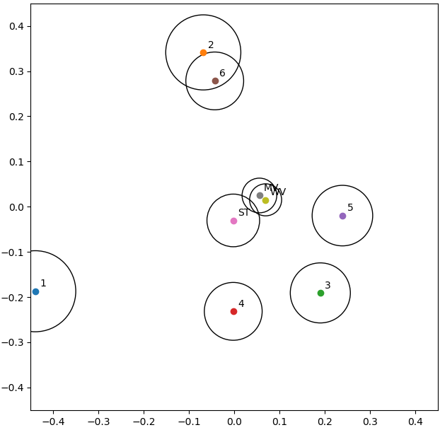
The results in Table 1 are averages computed from the head-to-head comparisons between experts, and those in Table 2 are comparisons with “ground truth” annotations, which also result from aggregations made by a consensus strategy. MDS allows us to clarify how the experts relate to each other and to the consensus methods, and these latter between them, as seen in Figure 3 : see updated/corrected version of the figure (Figure 7.8 in my PhD dissertation). It shows a slightly different relationship between the experts: "Experts 2 and 6 are “identical” in their head-to-head comparison, but their annotations only overlap on a few examples, so their distance to all other points are very different (hence the relatively large circles in the MDS plot). Between the four experts that provided more annotations (1, 3, 4 and 5), Experts 3 and 5 are often in agreement, but Expert 1 clearly appears as an outlier." --AF . The three consensus methods are very close to each other. Experts 2 and 6 form a tight cluster which counterbalances the loosest cluster of experts 3-4-5. This may explain why some agreement levels are more affected by the “leave-one-out” method. Indeed, whatever the method used, the consensus is mostly related to the loosest cluster, which, unlike the other cluster, groups experts with a high number of annotated maps. Expert 1 appears to be an outlier, which is interesting to note because this expert was used as a single source of ground truth in one of the publications using the dataset [24].
Such visualization provides an interesting opportunity for discussing the results of an algorithm. In challenges such as Gleason2019, the algorithms are ranked based on their similarity to the consensus. Computing a dissimilarity metric to each expert in addition to its calculation between experts and applying MDS on the resulting data would allow for a much finer analysis of the results and the algorithms’ behaviors. Specifically, it would indicate if an algorithm is located among the different experts, and therefore within the range of expert disagreement. It may also be possible to detect if an algorithm was more influenced by some experts.
While in a challenge it’s easy to produce a ranking of algorithms with the assumption of a single ground truth against which all algorithms are evaluated (but with several issues [2]), this approach greatly and unrealistically simplifies the complex and subjective nature of many digital pathology tasks. We would gain significant information by always keeping all the available annotations and giving a fair comparison between the algorithms and the different human experts. This would give room for a richer discussion of the results more in line with the clinical reality and complexity of the application.
Visualization techniques such as the one proposed here further provides an intuitive way of representing the results and make the detection of interesting patterns more obvious, both as an analysis of the dataset and these annotations, and as a comparison of results given by different algorithms. Our experiments show that the choice of the consensus method and the exact implementation of the core-level scoring rules affect the measured agreement, which may in turn influence the rankings of algorithms measured against this consensus. This affects the perception we may get from results, as broader agreement can be achieved through small changes in the implementation, and makes it difficult to compare results from sources where the exact implementation is not known.
It is therefore important for challenges to not only be transparent about how their ground truth was produced, but also to provide all the data required to be able to reproduce the published results, including individual annotation maps when available, consensus maps, and details on how other components of the challenge metrics (such as the core-level scores) were obtained : we go a lot more into that in our 2023 CMIG paper --AF .
Another interesting component of a challenge to analyse is the impact of the performance or agreement metric. The Gleason2019 challenge, for instance, may get different results if it replaces the unweighted with the quadratic kappa or, preferably, the linear kappa (less impacted by the number of categories), or if it uses a per-pixel metric less subject to class imbalance biases than the F1-score [26]. This will be explored in future work.