Introduction

Digital pathology produces very large images with a large amount of objects of interests of all scales and shapes. Most machine learning algorithms, particularly Deep Learning techniques, rely on large amounts of supervised data to find correct solutions. These data are hard to get, focusing most of the published work on a small set of good datasets used for challenges and benchmarks. It is however hard to judge how well these methods can perform on real-world, less accurate data. Being able to use imperfect data and still produce good results is an important challenge for DL. Imperfect data can take many different forms. In this work we will focus on errors in the annotations, while errors in image acquisition or other data corruption are not considered 24-02-09: we did study artifact segmentation in two papers: our Cloud'Tech 2018 paper and our follow-up report extending this publication. --AF . We first explore the different ways annotations can be described as “imperfect,” using classical ML paradigms. We measure how different types of error affect the results of a DL algorithm. We then implement methods adapted from those paradigms to reduce the errors and evaluate their performance.

Related Works

The study of the different imperfections of an annotated dataset has taken different forms in Machine Learning.

Semi-supervised learning (SSL) describes the case where a large part of the dataset lacks labels, but the available annotations are correct. Semi-supervised methods will typically use the unlabeled examples to estimate the shape of the data distribution, while the labeled data is used to separate the classes within that distribution [1]. The main assumptions of SSL are local-consistency (similar samples share the same label) and exotic-inconsistency (non-similar samples have different labels) [2]. Semi-supervised versions of classical ML algorithms have been developed, such as SVM [3] or Random Forests [4].

Weak learning (WL) is a relatively wide term which is generally linked with the idea that the desired output of the system is more precise than the available supervision. A typical example in image analysis is when image-level labels are provided, but the desired output is pixel-level segmentation. The classical framework for WL is Multiple Instance Learning (MIL) [5], [6]. In MIL, the instances (pixels) are unlabeled, but grouped per labeld bags (images). DL methods address this problem using deep convolutional neural networks (DCNN). In these DCNN the feature maps from different levels can be combined to provide segmentation, with a pooling method used to generate one single score per class at the network output for learning [7], [8].

Noisy datasets (ND) are cases where the supervision exists, but contains errors. In the present paper, we focus on labeling errors, i.e. the class allocated to the training example [9]. This label noise can be characterized by the noise transition matrix, which describes the probability for a given label to be mistaken with another [10]. Methods to use noisy data will be dependent on the transition matrix, and one such method will be described in section 3.2.

Typical digital pathology problems can have characteristics from all those concepts. It is often relatively easy to get large, unsupervised datasets (for instance from whole-slide imaging), with only partial supervision. To get more supervision, the annotations may be done more quickly in a less accurate manner by a non-expert, and will therefore be rough and imprecise 24-02-09: as was the case in our Cloud'Tech 2018 paper. --AF . These datasets can be also seen as including noisy labels, with a highly asymmetrical noise transition matrix. For instance, if a whole slide is annotated for mitoses, or glands, the annotated objects are generally correct (although possibly rough), but a number of them may have been missed.

Materials and Methods

While DL algorithms are developed to deal with real-world semi-supervised, noisy, and/or weak (SNOW) datasets, it is very difficult to evaluate them and compare their result quantitatively, because it is difficult or impossible to have a sufficiently large “gold standard" test set corresponding to the actual application 24-02-09: as we later realized, this is really something that many challenges and publications don't take into account enough, as the uncertainty on the results (depending on the metric) can be very important. See eg our analysis of digital pathology segmentation challenges published in Computerized Medical Imaging and Graphics in 2023. --AF . We thus use the GlaS challenge contest dataset [11] as a starting point to study how the performance of a DL algorithm is affected by different types of annotation weakness, and to identify the best approaches to mitigate these effects. The GlaS dataset consists in images taken from H&E-stained slides of colorectal tissue samples, including tumors, and where glands are annotated. There are 85 images in the training set and 80 in the test set. The supervision provided is a pixel-precise segmentation of the glands. Both sets contain around 750 glands, taking up around 50% of the total surface of the images.

Dataset corruption

The weaknesses that we want to include in the dataset attempt to recreate the kinds of errors found in usual digital pathology problems. Those errors are of two main types: missing annotations and imprecise annotations.

To simulate missing annotations, a proportion \(p_N\) of the glands is entirely removed in every training image, making the annotations noisy. We test different values for \(p_N\) to determine how much the level of label noise affects the segmentation results.

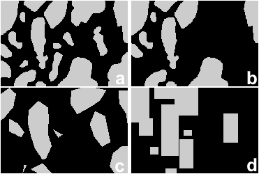
Imprecise annotations are modelled by deforming the objects in two different ways: size difference and shape approximation (polygonal or bounding box). Size difference simulates how people will naturally make an “outer contour" or an “inner contour" when annotating an image. It is done by performing morphological erosions and dilations using a disk kernel with a radius drawn from a normal distribution with standard deviation \(s_K\). Polygonal approximation relates to how quick annotations will be done with key points along the contour rather than following a pixel-precise “freehand" border, and produced by only keeping a fraction \(f_C\) of the border points to produce a simplified contour. Bounding boxes (BB) are another common way of producing quick annotations. Different corruption types are shown in Figure 1 24-02-09: SNOW generation code can be found on Github, although I don't remember if it's the exact version I used for this paper. I didn't have the good practice of keeping a snapshot of the code per publication when I wrote this one. --AF .

Baseline network and modifications

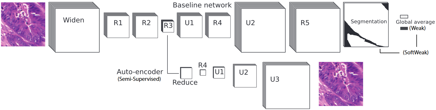
Our baseline network is a DCNN using residual units [12]. All convolutional layers use the Leaky ReLU activation function. A Softmax is applied after the last layer to get the final probability map of the segmentation. The network is trained using the cross-entropy cost function. This is a standard DCNN approach to solving a segmentation problem and serves as a reference to limit the variability. We modify this network and/or its training using different strategies related to the semi-supervised, noisy, and weak paradigms, as presented in Figure 2.

Positive examples. Using the baseline network, but trained only on the positive (which are mostly correct) examples, defined as patches which contain at least 80 pixels belonging to the “gland" class.

Semi-supervised (SS). An auto-encoder is trained on the full dataset without supervision (using the mean square error reconstruction cost). The weights in the first three residual units (R1 to R3 in Figure 2) are then used as the initialization for the training on the supervised set.

Weak. When the annotations are very imprecise, it can make more sense to use an image-level label instead of the full segmentation, and to trust the network to find which pixels were predictive of the target class. This is done by adding a global pooling layer after the segmentation 24-02-09: this worked well in our Artifact segmentation paper, but it really should have been obvious that it wasn't adapted to this particular dataset. Artifact in a WSI are sparse, but the GlaS data only focuses on regions with glands, so most tiles are "positive" (95% of extracted tiles, as we note in our follow-up). --AF .

SoftWeak (SW). This approach offers a compromise by using pixel-level annotations, possibly imprecise, combined with the image-level labels, both in the cost function and in the output prediction.

Noisy. The label noise introduced in the dataset is highly asymmetrical, in that it is much more likely that a “positive" example is mislabeled as “negative" (i.e. an object of interest is not annotated) than the opposite (i.e. a background region is mistakenly annotated). We therefore actually have only “positive and unannotated labels" [13]. The proposed solution is to treat unlabeled examples as both a positive and a negative example during training, either by duplicating the sample or by randomly choosing its label each time the sample is presented to the network.

We will also test different combinations of these methods.

Results

The metric used to compare the different methods and the effects of the weaknesses is the standard per-pixel \(F_1\) Score, defined as: \(F_1 = \frac{2 \times Precision \times Recall}{Precision+Recall}\) 24-02-09: aka Dice Similarity Coefficient, as it is more commonly called in segmentation tasks. --AF . We do not use the per-object score introduced in the GlaS contest because it is not useful for the more general comparison that interests us here 24-02-09: to use that, we would need to also implement post-processing to separate individual glands, which add anoter level of variability. --AF .

As the dataset is fairly small, basic data augmentation is done using mirroring, illumination change and random noise in the RGB levels 24-02-09: for an exploration of how much more thorough and realistic data augmentation can help with this dataset, see our colleague YR Van Eycke's 2018 study in Medical Image Analysis. --AF . Training is done on 256x256 pixels patches randomly taken from the training set images. For testing, we compute the prediction on the test image by tiling the patches with some overlap. The final value for a pixel is given by the maximum prediction from all patches which included this pixel. No post-processing is performed on the network predictions. The \(F_1\) scores are computed on all images of the GlaS test sets, using the full annotations. Prediction time is around 16ms per tile on a NVIDIA Titan X GPU.

Effects of noise and weaknesses

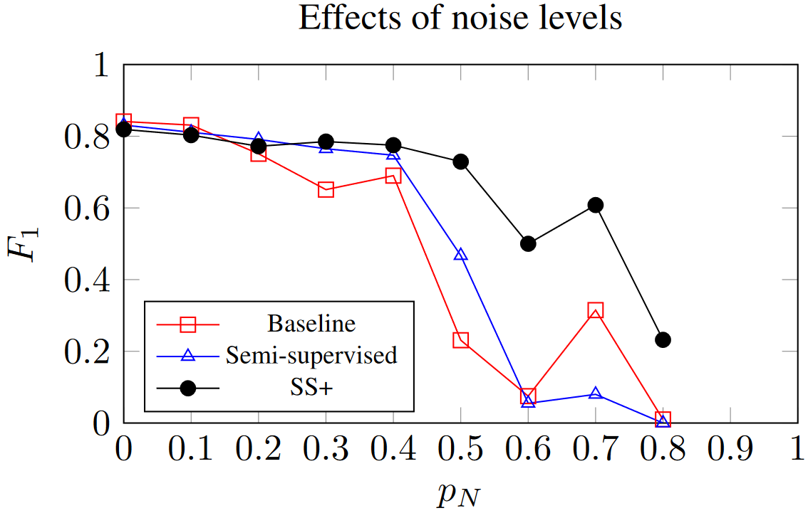
Figure 3 shows the effects of noise levels on the baseline network. Residual DCNNs show robustness to a limited amount of noise, but a sharp drop occurs around \(p_N=0.5\). We also observe that large deformations (HD set with \(s_K=20\) and \(f_C=80\)) only decrease the performance slightly (\(F_1=0.795\) compared to \(0.841\) on the full dataset) and that using only the bounding boxes has more impact (\(F_1=0.724\)). Finally, weakness combinations result in poor performances (HD+Noise: \(F_1=0.212\), BB+Noise: \(F_1=0.511\)).

Results of the proposed methods

All different and combined strategies are compared to the baseline network on the Noisy (\(p_N = 0.5\), where the performance drop occurs), BB, Noisy+BB and Noisy+HD sets. To objectively determine the best methods, we performed the Friedman test with post-hoc Nemenyi pair-wise tests on the test image scores. A summary of the results is shown in Table 1. Per dataset, the results in bold are not significantly different from the best one. For each data set, we characterize each method by the difference between the number of significantly worse methods and the number of significantly better method. On this basis, we propose a new statistical score for each method, which is the sum over all datasets of these differences 24-02-09: an implementation of this score can be found in my thesis code. --AF . The baseline network performs significantly worse than the other networks on the SNOW datasets. Overall, SS+ SoftWeak and Only Positive networks have the best performance, with SS+ not far behind. On the BB set Noisy SoftWeak and SS perform the best, but are unsatisfactory on the other sets.

Discussion and Future Work

Using artificial yet realistic imperfections in a dataset, we have quantified the effects of different annotation errors on the performance of a standard DL algorithm. Our results show that simple DCNN networks are robust to a certain amount of noise, but show an abrupt decrease in performances around the 50% noise mark. Deformations and imprecisions in the annotations also degrade the results significantly. Strategies adapted from classical machine learning can partially recover from this degradation. Our results suggest that it is often better to use a smaller dataset with few annotations errors ("only positive" strategy), possibly combined with unsupervised pre-training on a larger set (SS+ and SS+ SW strategy). Further work will study whether these results are confirmed on other weakened datasets, possibly with other DCNN networks, and will apply those insights to real-world SNOW datasets 24-02-09: see the "future work". --AF . We suspect that a network specialized in learning object edges (such as the winner of the GlaS contest [11]) will be particularly affected by annotation distortions such as BB and HD.

Acknowledgements

We gratefully acknowledge the support of NVIDIA Corporation with the donation of a Titan X Pascal GPU used in this study. The Center for Microscopy and Molecular Imaging (CMMI) is supported by the European Regional Development Fund and the Walloon Region [Wallonia-Biomed grant 411132-957270]. C.D. is a senior research associate with the National (Belgian) Fund for Scientific Research (FNRS).