Artefact detection in Digital Pathology

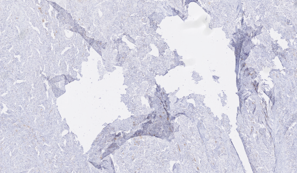
A digital pathology task that illustrates quite well the "imperfect nature of digital pathology annotations" that I mentioned in the previous post is artefact detection. In the first post of this blog, I presented the main steps of Digital Pathology, from the extraction of the tissue sample to the digitalization of the slide. Throughout this process, the tissue is manipulated, cut, moved, stained, cleaned, sometimes frozen, and more generally exposed to the elements. This can cause serious damage, as illustrated in the figure below. Sometimes, problems can also occur during the acquisition process, leading to blurriness or contrast issues.

Depending on the severity of those issues, we may have to discard parts of the image from further analysis, redo the acquisition process or, in extreme cases, require a new slide to be produced. This can have a big negative impact on the pathology workflow, and it is also a potential source of uncertainty on the results. Typically, this "quality control" is done manually. This can take a lot of time, and it is a very subjective process which can lead to many mistakes [1]. Some algorithms had been proposed in the past to detect some specific types of artefact, such as blurry regions [2] or tissue-folds [3], but our goal was to develop a general-purpose method to catch most artefacts in one pass.

The dataset

Whose slide images are very large. Artefacts can be of varying sizes and shapes, making them extremely tedious to annotate. This is a situation that will always lead to imperfect annotations. We had one slide annotated in details by an histology technologist, and even in that slide many of the annotations were missing, or imprecise. To be able to get enough data to train a neural network, I quickly annotated the rest of the dataset based on the technologist's example, and I'm not an expert at all. As a result, we had a dataset with annotations that were rough, didn't really match the contours of the artefacts, and where a lot of artefacts were not marked at all. We had 26 slides in total. Slides are very large images, so while twenty-six seems like a very low number for training a neural network, we can actually extract a very large number of smaller patches from those slides to satisfy our needs.

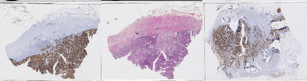
An interesting thing about the data is that it has different types of staining, as shown in the figure above. Some of the slides have been stained with a standard "Haematoxilyn & Eosin" treatment, which is typical to show the general morphology of the tissue, while others have been stained with immunohistochemistry biomarkers, highlighting tumoral tissue in brown.

One of the first question we always have to answer once we have a dataset is: what do we use to train our models, and what do we use to evaluate them?

In this case, as we had one slide with "better" annotations than the rest, we decided to keep it for testing. There were two good reasons for that: first, this would make the evaluation more likely to be meaningful; second, that slide came from another source and another staining protocol as the others, which would help us test the "generalization" capability of our methods.

What makes the difference?

The main thing we wanted to see was: what parts of the machine learning pipeline were really important, and had an impact on the results? What we initially did was to take a relatively small, straightforward neural network architecture, and to test many different small changes in its depth ("how many layers") and width ("how many neurons per layer"). We also looked at whether we should use different levels of magnification on the image, or if we should try to "balance" the dataset by sampling more artefacts, as they were more examples of normal tissue than of artefact tissue in the data. Finally, we tried to compare using a "segmentation" output (predicting for each pixel if there is an artefact or not) or a "detection" output (predicting for the whole image patch if there is an artefact or not).

We published our first results at the "CloudTech 2018" conference [4]. What we found most interesting was that, quite clearly, the details of the network architecture didn't really matter. The balance of the dataset and how we decided to produce our "per pixel" output (directly from the network, or by combining the detection results from overlapping patches) were the main factors that influenced the final results.

Let's have a look at this result, for instance:

Here, we have the same network, which uses patch-based detection, and has been trained using different data sampling. If we randomly sample the patches from the original dataset, we don't have enough examples of artefacts, and the network misses most of them. If we increase the percentage of artefact examples in the training batches, the network becomes a lot more sensitive. Obviously, this comes at the risk of falsely detecting normal tissue.

How can we evaluate those results?

Evaluation metrics have to be related to the usage that we want to make of the results. In this case, the goals can be to assess the "quality" of the slide (or: to know how much of the slide is corrupted), and to remove damaged areas from further processing. For the latter task, we can reformulate it as: finding the "good" areas that can be used later.

There is no single metric that can really give us all that information. We computed the accuracy (which proportion of the pixels were correctly classified), the "True Positive Rate" (which proportion of the annotated artefacts did we correctly identify), the "True Negative Rate" (which proportion of the normal tissue did we correctly identify), and the "Negative Predictive Value" (which proportion of the tissue we identified as normal is actually normal). A low TPR would mean that we missed many artefacts; a low TNR that we removed a large portion of normal tissue; a low NPV that our "normal tissue" prediction is unreliable. To take the subjective nature of the evaluation into account, we also added a simple qualitative assessment, which we formulated as a binary choice: could this result be reasonably used in a digital pathology pipeline?

None of those metrics were really satisfactory. The trend that "what goes around the network" had a lot more impact than minute changes within, however, was clear enough that we could draw useful conclusions from those first experiments.

The main lesson

These first experiments with artefact detection showed that the way we prepared our dataset, and the way we defined our problem, had more impact on our results than the network itself. This is particularly visible when working on a dataset with very imperfect annotations, where just fitting the raw data into a deep learning model will lead to extremely poor results.

A lot of published research in computer vision for digital pathology is done on datasets published in challenges. These datasets tend to be very "clean", with precise annotations and pre-selected regions of interest. This makes it easier to train machine learning models, and it also makes it a lot easier to test and compare algorithms with one another. But the question we wanted to explore now was: as real-world datasets from research or clinical practice are not generally as clean as challenge datasets, shouldn't we be cautious about the conclusions we draw from these challenge results?

References

• [↑] A. Janowczyk et al. (2019) "HistoQC: An Open-Source Quality Control Tool for Digital Pathology Slides", JCO Clinical Cancer Analytics, DOI: 10.1200/CCI.18.00157
• [↑] X. Moles Lopez et al. (2012) "An Automated Blur Detection Method for Histological Whole Slide Imaging", PLoS One 8(12), DOI: 10.1371/journal.pone.0082710
• [↑] A. Kothari et al. (2013) "Eliminating tissue-fold artifacts in histopathological whole-slide images for improved image-based prediction of cancer grade", Journal of Pathology Informatics 4:22, DOI: 10.4103/2153-3539.117448
• [↑] A. Foucart et al. (2018) "Artifact Identification in Digital Pathology from Weak and Noisy Supervision with Deep Residual Networks", Proc. CloudTech 2018, DOI: 10.1109/CloudTech.2018.8713350